[deep learning]: day 8 of pytorch introduction to project practice: weight decline (including source code)

【 Deep learning 】：《PyTorch Introduction to project practice 》 Eighth days ： Weight decline （ Including source code ）

• This article is included in 【 Deep learning 】：《PyTorch Introduction to project practice 》 special column , This column mainly records how to use PyTorch Realize deep learning notes , Try to keep updating every week , You are welcome to subscribe ！
• Personal home page ：JoJo Data analysis adventure
• Personal introduction ： I'm reading statistics in my senior year , At present, Baoyan has reached statistical top3 Colleges and universities continue to study for Postgraduates in Statistics
• If it helps you , welcome Focus on 、 give the thumbs-up 、 Collection 、 subscribe special column

Reference material ： This column focuses on bathing God 《 Hands-on deep learning 》 For learning materials , Take notes of your study , Limited ability , If there is a mistake , Welcome to correct . At the same time, Musen uploaded teaching videos and teaching materials , You can go to study .

• video ： Hands-on deep learning
• The teaching material ： Hands-on deep learning

1. Basic concepts

In the previous section, we described the problem of over fitting , Although we can reduce over fitting by adding more data , But the cost is higher , Sometimes it's not enough . So now let's introduce some regularization methods . In deep learning , Weight decay is a widely used regularization method . The principle is as follows .
We introduce L2 Regularization , At this point, our loss function is ：
$$\frac{1}{2m}\sum _{i=1}^n(W^T{X}^{(i)}+b-y^{(i)}{)}^2+\frac{\lambda }{2}||W|{|}^2$$
among ,$\frac{\lambda }{2}||W|{|}^2$ It's called a penalty item
The gradient of the new function at any time is obtained ：
$$\frac{dL}{dw}+\lambda W$$
As we updated the parameters before ,L2 The gradient descent of regularized regression is updated as follows ：
$$w:=(1-\eta \lambda )w-\eta \frac{dL}{dw}$$
Usually $\eta \lambda <1$, So in deep learning we call it weight decay .
matters needing attention ：

• 1. We are only concerned with weights W To punish , Not right b To punish
• 2.$\lambda$ It's a super parameter , The bigger the value is. , The greater the decline in weight , As we approach infinity , Weight approach 0, Conversely, if the value is 0, There is no constraint .
• 3.L2 Regularization cannot achieve sparse results , If you want to reduce features , Use L1 Regularization for feature selection .
  Let's take a look at how it is implemented through specific code

2. Code implementation

As in the previous chapter , Use analog datasets as usual , The generated data set is as follows ：
$$y=0.1+\sum _{i=1}^{d}0.01x_i+ϵ\text{ where }ϵ\sim \mathcal{N}(0,0.01^2)$$

2.1 Generate data set

Here we assume that the real data are as follows ：
$$y=0.1+\sum _{i=1}^{200}0.01x_i+ϵ$$
Let's make a data set

""" Import related libraries """
import torch
from d2l import torch as d2l
from torch import nn
%matplotlib inline

#  Define correlation functions . This is the function in Mu Shen's textbook , If you download d2l You can import 
def synthetic_data(w, b, num_examples):  #@save
    """ Generate y=Xw+b+ noise """
    X = torch.normal(0, 1, (num_examples, len(w)))
    y = torch.matmul(X, w) + b
    y += torch.normal(0, 0.01, y.shape)
    return X, y.reshape((-1, 1))
def load_array(data_arrays, batch_size, is_train=True): 
    """ Construct a PyTorch Data iterators """
    dataset = data.TensorDataset(*data_arrays)# Convert data to tensor
    return data.DataLoader(dataset, batch_size, shuffle=is_train)

""" Generate data set """
n_train, n_test, num_inputs, batch_size = 50, 100, 200, 5# Define related training sets , Verification set , The input variable , as well as batch Size 
true_w, true_b = torch.ones((num_inputs, 1)) * 0.01, 0.1# Define real parameters 
train_data = d2l.synthetic_data(true_w, true_b, n_train)# Generate simulation data , The specific functions are as follows 
train_iter = d2l.load_array(train_data, batch_size)# Load training set data 
test_data = d2l.synthetic_data(true_w, true_b, n_test)
test_iter = d2l.load_array(test_data, batch_size, is_train=False)

According to the introduction in the previous chapter , We know that the smaller the sample, the easier it is to cause over fitting , Here we set the sample size to 100, But the parameters have 200 individual , In this case p>n, It is easy to cause over fitting .

2.2 Initialize parameters

After generating the dataset , The next step is to initialize the parameters , Here we are talking about weights $w$ Initialize to standard normal distribution , deviation $b$ Initialize to 0

def init_params():
    w = torch.normal(0, 1, size=(num_inputs, 1), requires_grad=True)# Generate standard normal distribution 
    b = torch.zeros(1, requires_grad=True)# Generate all for 0 The data of 
    return [w, b]

2.3 Define penalty items

Here we define L2 Regularization , The specific code is as follows

def l2_penalty(w):
    return torch.sum(w.pow(2)) / 2

2.3 Training

This is basically the same as the previous linear regression training , The only difference is that there is one more penalty item , therefore lambd Is a super parameter

def train(lambd):
    w, b = init_params()# Initialize parameters 
    net, loss = lambda X: d2l.linreg(X, w, b), d2l.squared_loss# Anonymous functions are used here , Two functions are defined , One is the result of solving the model , One is the loss function 
    num_epochs, lr = 100, 0.003
    """ Define relevant graphic settings """
    animator = d2l.Animator(xlabel='epochs', ylabel='loss', yscale='log',
                            xlim=[5, num_epochs], legend=['train', 'test'])
    """ model training , Update parameters """
    for epoch in range(num_epochs):
        for X, y in train_iter:
            #  Added L2 Norm penalty term ,
            #  The broadcasting mechanism makes l2_penalty(w) Become a length of batch_size Vector 
            l = loss(net(X), y) + lambd * l2_penalty(w)
            l.sum().backward()
            d2l.sgd([w, b], lr, batch_size)
        """ Draw training error and test error """
        if (epoch + 1) % 5 == 0:
            animator.add(epoch + 1, (d2l.evaluate_loss(net, train_iter, loss),
                                     d2l.evaluate_loss(net, test_iter, loss)))
    print('w Of L2 Norm is ：', torch.norm(w).item())

First , Let's take a look at the case of not adding penalties , That is, it is consistent with our previous linear regression , here , Serious over fitting , As shown in the figure below

train(lambd=0)

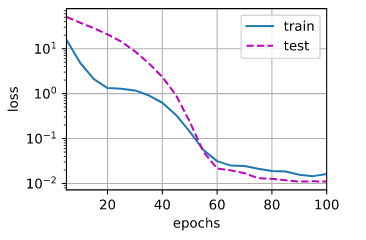
From the results above , There is a serious over fitting problem , The verification error is much larger than the training error . Let's take a look at lambd by 5 The result of the case

train(lambd=5)

It can be seen that , With lambd An increase in , Verification error is decreasing , But there is still a fitting .

def train_concise(wd):
    net = nn.Sequential(nn.Linear(num_inputs, 1))# Define linear neural networks 
    for param in net.parameters():
        param.data.normal_()# Initialize parameters 
    loss = nn.MSELoss(reduction='none')# Definition MSE Loss function 
    num_epochs, lr = 100, 0.003# Define training times and learning rates 
    #  The offset parameter has no attenuation 
    trainer = torch.optim.SGD([
        {
    "params":net[0].weight,'weight_decay': wd},
        {
    "params":net[0].bias}], lr=lr)# Define weight decay , Where the super parameter is wd
    animator = d2l.Animator(xlabel='epochs', ylabel='loss', yscale='log',
                            xlim=[5, num_epochs], legend=['train', 'test'])# mapping 
    """ Training models """
    for epoch in range(num_epochs):
        for X, y in train_iter:
            trainer.zero_grad()
            l = loss(net(X), y)
            l.mean().backward()
            trainer.step()
        if (epoch + 1) % 5 == 0:
            animator.add(epoch + 1,
                         (d2l.evaluate_loss(net, train_iter, loss),
                          d2l.evaluate_loss(net, test_iter, loss)))
    print('w Of L2 norm ：', net[0].weight.norm().item())

train_concise(0)

train_concise(3)

3. Expansion part

Mu Shen's reference textbook uses L2 Regularization , Let's look at using L1 The effect of regularization , First, we need to define L1 Regularization , As shown below ：
$$\frac{1}{2m}\sum _{i=1}^n(W^T{X}^{(i)}+b-y^{(i)}{)}^2+\lambda |W|$$

def l1_penalty(w):
    return torch.sum(torch.abs(w))

def train_l1(lambd):
    w, b = init_params()# Initialize parameters 
    net, loss = lambda X: d2l.linreg(X, w, b), d2l.squared_loss# Anonymous functions are used here , Two functions are defined , One is the result of solving the model , One is the loss function 
    num_epochs, lr = 100, 0.003
    """ Define relevant graphic settings """
    animator = d2l.Animator(xlabel='epochs', ylabel='loss', yscale='log',
                            xlim=[5, num_epochs], legend=['train', 'test'])
    """ model training , Update parameters """
    for epoch in range(num_epochs):
        for X, y in train_iter:
            #  Added L1 Norm penalty term ,
            #  The broadcasting mechanism makes l1_penalty(w) Become a length of batch_size Vector 
            l = loss(net(X), y) + lambd * l1_penalty(w)
            l.sum().backward()
            d2l.sgd([w, b], lr, batch_size)
        """ Draw training error and test error """
        if (epoch + 1) % 5 == 0:
            animator.add(epoch + 1, (d2l.evaluate_loss(net, train_iter, loss),
                                     d2l.evaluate_loss(net, test_iter, loss)))
    print('w Of L2 Norm is ：', torch.norm(w).item())

train_l1(1)

It can be seen that the L1 Regularization , When lambd by 1 When , The verification error is basically equal to the training error . In fact, as we said before ,L2 Regularization can only compress parameters , But it cannot be removed as 0, Our simulation dataset ,p by 200,n by 100,p>>n, At this time to use L1 Regularization can make the coefficients of some features be 0, So as to better alleviate the over fitting problem .

This is the introduction of this chapter , If it helps you , Please do more thumb up 、 Collection 、 Comment on 、 Focus on supporting ！！