当前位置:网站首页>Time series analysis 41 - time series prediction tbats model
Time series analysis 41 - time series prediction tbats model
2022-07-28 09:49:00 【Magic Ktwc37】
Timing analysis 41
Timing prediction TBATS Model
We introduced (S)ARIMA(X) Series model 、Prophet And other methods to predict time series data , In this article, we try to use TBATS Model for time series prediction .TBATS The main goal of the model is to model complex seasonal factors in an exponential smoothing way . Please look at the chart below. ,
TBATS: Trigonometric seasonality, Box-Cox transformation, ARMA errors, Trend and Seasonal components.
brief introduction
Generally speaking, the problem of time series prediction is to predict the future value of time series according to the historical observations of the time series data . In the process of modeling, one of the headache problems of menstruation is the uncertainty of time series , It changes according to the data scenario .
And this article will introduce TBATS The model mainly uses exponential smoothing method to solve complex periodic problems .
TBATS Different options will be considered to model the period of time series , Include :
- Conduct Box-Cox Convert and do not Box-Cox transformation
- Consider timing trends and ignore trends
- Use trend attenuation and inapplicable trend attenuation
- Use for model residuals ARIMA(p,q) Or not
- No seasonal model
- Balance seasonal factors to varying degrees
Please look at the chart below. :
The final model selection uses Akaike information (AIC, Akaike information criterion).
Be careful : Automatically ARIMA It is used to determine whether the residuals need modeling or find appropriate parameters (p,q).
A simple example
Let's take a look at the simplest example
from tbats import TBATS
import numpy as np
# required on windows for multi-processing,
# see https://docs.python.org/2/library/multiprocessing.html#windows
if __name__ == '__main__':
    np.random.seed(2342)
    t = np.array(range(0, 160))
    y = 5 * np.sin(t * 2 * np.pi / 7) + 2 * np.cos(t * 2 * np.pi / 30.5) + \
        ((t / 20) ** 1.5 + np.random.normal(size=160) * t / 50) + 10

    # Create estimator
    estimator = TBATS(seasonal_periods=[14, 30.5])

    # Fit model
    fitted_model = estimator.fit(y)

    # Forecast 14 steps ahead
    y_forecasted = fitted_model.forecast(steps=14)

    # Summarize fitted model
    print(fitted_model.summary())
Use Box-Cox: True
Use trend: True
Use damped trend: True
Seasonal periods: [14. 30.5]
Seasonal harmonics [2 1]
ARMA errors (p, q): (0, 0)
Box-Cox Lambda 0.654044
Smoothing (Alpha): 0.132425
Trend (Beta): 0.023495
Damping Parameter (Phi): 0.947184
Seasonal Parameters (Gamma): [-9.18866163e-09 -4.37211750e-09 -1.04956292e-08 -1.81209981e-08]
AR coefficients []
MA coefficients []
Seed vector [ 5.69510575e+00 -1.36715628e-01 4.70120645e-04 4.91577774e-02
-3.14318406e-02 1.93662153e+00 6.22414387e-01 9.31711655e-02]
AIC 1028.837243
# Time series analysis
print(fitted_model.y_hat) # in sample prediction
print(fitted_model.resid) # in sample residuals
print(fitted_model.aic)
[12.00026315 15.37130609 15.92513946 12.92209113 8.86829808 6.55044357
6.98379669 9.80510678 12.96461526 13.46459656 10.73401852 6.96869927
4.88388936 5.2411647 7.89921391 11.16766831 12.01242589 9.84585836
6.61337902 4.99937038 5.90163047 9.22357233 13.21064516 14.63622867
12.54077865 9.32236216 7.62704064 8.86253335 12.72529442 16.732014
17.97565652 15.35674111 11.53204899 9.35938536 10.22652865 13.76843469
…
[-2.63150260e-04 4.92298548e-01 7.81058008e-01 1.04674185e+00
4.74485095e-01 -2.89650437e-01 -1.09380563e-02 7.11659349e-01
7.52445725e-01 1.52818057e+00 7.74776582e-01 2.21684967e-01
-1.03614988e+00 -3.83613709e-01 1.26200022e+00 1.11129016e+00
2.11411936e+00 9.74278300e-01 5.82900889e-01 -3.77720695e-01
-1.42384359e-01 1.28154205e+00 1.23632142e+00 9.87393000e-01
1.61135725e+00 5.23587924e-01 3.71403105e-01 4.83700871e-01
…
1028.8372428992702
# Reading model parameters
print(fitted_model.params.alpha)
print(fitted_model.params.beta)
print(fitted_model.params.x0)
print(fitted_model.params.components.use_box_cox)
print(fitted_model.params.components.seasonal_harmonics)
0.13242488070375835
0.023495267045578822
[ 5.69510575e+00 -1.36715628e-01 4.70120645e-04 4.91577774e-02
-3.14318406e-02 1.93662153e+00 6.22414387e-01 9.31711655e-02]
True
[2 1]
A more complicated example
We still use the front SARIMAX Data used in the series of blog posts , This data is a daily sales data , contain 5 year 10 In storage 50 Sales data of products . In this example, we use warehousing 1 Products in 1 related data .
import pandas as pd
df = pd.read_csv('walmart/train.csv')
df = df[(df['store'] == 1) & (df['item'] == 1)] # item 1 in store 1
df = df.set_index('date')
y = df['sales']
y_to_train = y.iloc[:(len(y)-365)]
y_to_test = y.iloc[(len(y)-365):] # last year for testing

We can see the weekly and annual periodicity in the figure , This indicates that there are multiple cycles in the sequence
TBATS Model
from tbats import TBATS, BATS # Fit the model
estimator = TBATS(seasonal_periods=(7, 365.25))
model = estimator.fit(y_to_train)# Forecast 365 days ahead
y_forecast = model.forecast(steps=365)
Note that the annual cycle is defined as 365,25, Not an integer , But it doesn't matter ,TBATS The model can be supported .
it seems ,TBATS The model fits well for two kinds of mixed periodicity .
Annual periodic fitting 
Weekly periodic fitting
The model parameters are as follows :
Use Box-Cox: True
Use trend: False
Use damped trend: False
Seasonal periods: [ 7. 365.25]
Seasonal harmonics [ 3 11]
ARMA errors (p, q): (0, 0)
Box-Cox Lambda 0.234955
Smoothing (Alpha): 0.015789
TBATS Three equilibrium strategies are used for weekly periodicity , For annual periodicity 11 An equilibrium strategy ; At the same time Box-Cox Method ,lambda by 0.234955; There is no trend modeling , Not used ARMA Modeling residuals .
SARIMA Model weekly periodicity
SARIMA Only one cycle can be modeled , And the cycle cannot be too long . Let's try to use SARIMA Model the time series data , It can be done with TBATS Compare the .
from pmdarima import auto_arima
arima_model = auto_arima(y_to_train, seasonal=True, m=7)
y_arima_forecast = arima_model.predict(n_periods=365)
Autoarima I chose SARIMA(0, 1, 1)x(1, 0, 1, 7) model, Annual periodicity is not modeled .
SARIMAX + Fourier term
We can use SARIMAX Model , Take Fourier term as external variable to fit the second periodic factor .
# prepare Fourier terms
exog = pd.DataFrame({
    'date': y.index})
exog = exog.set_index(pd.PeriodIndex(exog['date'], freq='D'))
exog['sin365'] = np.sin(2 * np.pi * exog.index.dayofyear / 365.25)
exog['cos365'] = np.cos(2 * np.pi * exog.index.dayofyear / 365.25)
exog['sin365_2'] = np.sin(4 * np.pi * exog.index.dayofyear / 365.25)
exog['cos365_2'] = np.cos(4 * np.pi * exog.index.dayofyear / 365.25)
exog = exog.drop(columns=['date'])
exog_to_train = exog.iloc[:(len(y)-365)]
exog_to_test = exog.iloc[(len(y)-365):]# Fit model
arima_exog_model = auto_arima(y=y_to_train, exogenous=exog_to_train, seasonal=True, m=7)# Forecast
y_arima_exog_forecast = arima_exog_model.predict(n_periods=365, exogenous=exog_to_test)
Here we use two Fourier terms as external variables . Now? SARIMAX The model completes the modeling of two cyclical factors .
Model comparison
We use Mean Absolute Error Compare the three models :
TBATS: 3.8527
SARIMA:7.2249
SARIMAX + 2 Fourier term :3.9045
Advantages and disadvantages
advantage
TBATS The model can model complex cyclical factors , Such as non integer period 、 Long period, etc .
shortcoming
because TBATS The model mixes and tries many methods at the bottom , So its calculation speed is relatively slow .
TBATS The model cannot be like SARIMAX Add external variables like that .
边栏推荐
- Business visualization - make your flowchart'run'(4. Actual business scenario test)
- 软件测试与质量学习笔记1---黑盒测试
- [collection] linear algebra let me think - Summary of chapter topics
- Salted fish esp32 instance - mqtt lit LED
- Window源码解析(二):Window的添加机制
- Source code analysis of view event distribution mechanism
- Arouter source code analysis (I)
- MATLAB的实时编辑器
- Translation recommendation | debugging bookkeeper protocol - unbounded ledger
- ECCV 2022 | can be promoted without fine adjustment! Registration based anomaly detection framework for small samples
猜你喜欢

初学C#必须要掌握的基础例题

NET 3行代码实现文字转语音功能

MySQL中各类型文件详解
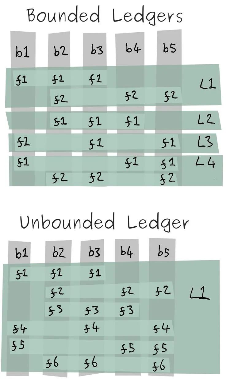
译文推荐 | 调试 BookKeeper 协议 - 无界 Ledger

pycharm使用conda调用远程服务器

C# 倒计时工具

MySQL master-slave architecture. After the master database is suspended and restarted, how can the slave database automatically connect to the master database

MATLAB的实时编辑器

Business visualization - make your flowchart'run'(4. Actual business scenario test)
Edge团队详解如何通过磁盘缓存压缩技术提升综合性能体验

随机推荐
Buckle 376 swing sequence greedy
ActivityRouter源码解析
Real time editor of MATLAB
Opencv installation configuration test
Arouter source code analysis (I)
数据库高级学习笔记--存储函数
SQL server, MySQL master-slave construction, EF core read-write separation code implementation
MATLAB的符号运算
PlatoFarm进展不断,接连上线正式版以及推出超级原始人NFT
Plato Farm-以柏拉图为目标的农场元宇宙游戏
Machine learning (10) -- hypothesis testing and regression analysis
MATLAB的数列与极限运算
数据库高级学习笔记--游标
Scalable search bar, imitating Huawei application market
TimeBasedRollingPolicy简介说明
Opencv4.60 installation and configuration
软件测试与质量学习笔记1---黑盒测试
NET 3行代码实现文字转语音功能
实验四 使用fdisk对硬盘进行管理
数据库那么多概念性的东西怎么学?求方法