当前位置:网站首页>Chinese Version Vocaloid AI Tuner Feasibility Test
Chinese Version Vocaloid AI Tuner Feasibility Test
2022-06-12 01:19:00 【Yangsier】
The purpose of this test is to show that there is correlation between modifiable argument in Vocaloid project file and quality of tuning.
What is Vocaloid? Here is a link to wiki page.
Vocaloid:
Vocaloid (ボーカロイド, Bōkaroido) is a singing voice synthesizer software product. Its signal processing part was developed through a joint research project led by Kenmochi Hideki at the Pompeu Fabra University in Barcelona, Spain, in 2000 and was not originally intended to be a full commercial project. Backed by the Yamaha Corporation, it developed the software into the commercial product “Vocaloid” which was released in 2004.
Project github repo: https://github.com/Discover304/AI-Tuner
Prepare dataset
In this part we will get a formated vsqx data in dictionary with 2 dimension infromation note and id.
- import vocaloid project (.vsqx) and extract all test related arguments (arg)
- format all args to 960 length list where 960 is the time stamps
# adding path to system
import sys, os
sys.path.append(os.getcwd())

# read the data index json file
import json
dataPath = os.path.join(os.getcwd(), 'VocaloidVSQXCollection')
with open(os.path.join(dataPath,"source.json"), 'r',encoding='utf-8') as f:
    source = json.load(f) # source is a dictionary
fileList = [source[sourceIndex]["file"] for sourceIndex in range(len(source))]

[print(str(sourceIndex+1) + ". Thanks for the data from creator: " + source[sourceIndex]["creator"] + "\n\tSource of data: " + source[sourceIndex]["website"] + "\n") for sourceIndex in range(len(source))]

# initialise all reoslvers
from vocaloidDao import vocaloidVSQXResolver
resolverList = [vocaloidVSQXResolver(os.path.join(dataPath, fileName)) for fileName in fileList]
1. Thanks for the data from creator: Mixing : リサRisa Source of data: https://www.vsqx.top/project/vn1801 2. Thanks for the data from creator: Grill the music : Star sunflower / Mixing :seedking Source of data: https://www.vsqx.top/project/vn1743 3. Thanks for the data from creator: N/A Source of data: https://www.vsqx.top/project/vn1784 4. Thanks for the data from creator: vsqx:DZ Wei Yuanzi Source of data: https://www.vsqx.top/project/vn1752 5. Thanks for the data from creator: N/A Source of data: https://www.vsqx.top/project/vn1749 6. Thanks for the data from creator: Fill in the words ~ Super supervised crow , Ode to the Millennium recipe vsqx~ Say , Make ~cocok7 Source of data: https://www.vsqx.top/project/vn1798 7. Thanks for the data from creator: Accompaniment : Ono road ono (https://www.dizzylab.net/albums/d/dlep02/) Source of data: https://www.vsqx.top/project/vn1788 8. Thanks for the data from creator: transfer / mixed : Evil cloud Grill the music : Oh, my God, my string Source of data: https://www.vsqx.top/project/vn1796 9. Thanks for the data from creator: Grill the music : Phosphorus P Source of data: https://www.vsqx.top/project/vn1753 10. Thanks for the data from creator: N/A Source of data: https://www.vsqx.top/project/vn1778
# resolve all original data in parallel way, and save them to loacl
from vocaloidDao import parallelResolve
print("It may take a while if the file are resolved for the first time.")
parallelResolve(resolverList)
It may take a while if the file are resolved for the first time. local computer has: 16 cores Parallal computing takes 0.00 seconds to finish.
# load saved data
VocaloidDataDfs = [resolver.loadFormatedVocaloidData() for resolver in resolverList]

# import as dataframe
import pandas as pd
VocaloidDataDf = pd.DataFrame()
for VocaloidDataDfIndex in range(len(VocaloidDataDfs)):
    VocaloidDataDf = VocaloidDataDf.append(VocaloidDataDfs[VocaloidDataDfIndex])
VocaloidDataDf = VocaloidDataDf.reset_index()
VocaloidDataDf.head()
Log: loaded Log: loaded Log: loaded Log: loaded Log: loaded Log: loaded Log: loaded Log: loaded Log: loaded Log: loaded
.dataframe tbody tr th:only-of-type { vertical-align: middle; } <pre><code>.dataframe tbody tr th { vertical-align: top; } .dataframe thead th { text-align: right; } </code></pre>
index | D | G | W | P | S | VEL | T | OPE | DUR | |
|---|---|---|---|---|---|---|---|---|---|---|
0 | 0 | [0, 0, 0, 0, 0, 0, 0, 0, 0, 0, 0, 0, 0, 0, 0, ... | [0, 0, 0, 0, 0, 0, 0, 0, 0, 0, 0, 0, 0, 0, 0, ... | [0, 0, 0, 0, 0, 0, 0, 0, 0, 0, 0, 0, 0, 0, 0, ... | [0, 0, 0, 0, 0, 0, 0, 0, 0, 0, 0, 0, 0, 0, 0, ... | [0, 0, 0, 0, 0, 0, 0, 0, 0, 0, 0, 0, 0, 0, 0, ... | [64, 64, 64, 64, 64, 64, 64, 64, 64, 64, 64, 6... | [0, 1, 2, 3, 4, 5, 6, 7, 8, 9, 10, 11, 12, 13,... | [127, 127, 127, 127, 127, 127, 127, 127, 127, ... | [90, 90, 90, 90, 90, 90, 90, 90, 90, 90, 90, 9... |
1 | 1 | [0, 0, 0, 0, 0, 0, 0, 0, 0, 0, 0, 0, 0, 0, 0, ... | [0, 0, 0, 0, 0, 0, 0, 0, 0, 0, 0, 0, 0, 0, 0, ... | [0, 0, 0, 0, 0, 0, 0, 0, 0, 0, 0, 0, 0, 0, 0, ... | [0, 0, 0, 0, 0, 0, 0, 0, 0, 0, 0, 0, 0, 0, 0, ... | [0, 0, 0, 0, 0, 0, 0, 0, 0, 0, 0, 0, 0, 0, 0, ... | [64, 64, 64, 64, 64, 64, 64, 64, 64, 64, 64, 6... | [0, 1, 2, 3, 4, 5, 6, 7, 8, 9, 10, 11, 12, 13,... | [127, 127, 127, 127, 127, 127, 127, 127, 127, ... | [30, 30, 30, 30, 30, 30, 30, 30, 30, 30, 30, 3... |
2 | 2 | [64, 64, 64, 64, 64, 64, 64, 64, 64, 64, 64, 6... | [0, 0, 0, 0, 0, 0, 0, 0, 0, 0, 0, 0, 0, 0, 0, ... | [0, 0, 0, 0, 0, 0, 0, 0, 0, 0, 0, 0, 0, 0, 0, ... | [2418, 2418, 2418, 2418, 2418, 2418, 2418, 241... | [0, 0, 0, 0, 0, 0, 0, 0, 0, 0, 0, 0, 0, 0, 0, ... | [64, 64, 64, 64, 64, 64, 64, 64, 64, 64, 64, 6... | [0, 1, 2, 3, 4, 5, 6, 7, 8, 9, 10, 11, 12, 13,... | [127, 127, 127, 127, 127, 127, 127, 127, 127, ... | [150, 150, 150, 150, 150, 150, 150, 150, 150, ... |
3 | 3 | [0, 0, 0, 0, 0, 0, 0, 0, 0, 0, 0, 0, 0, 0, 0, ... | [0, 0, 0, 0, 0, 0, 0, 0, 0, 0, 0, 0, 0, 0, 0, ... | [0, 0, 0, 0, 0, 0, 0, 0, 0, 0, 0, 0, 0, 0, 0, ... | [0, 0, 0, 0, 0, 0, 0, 0, 0, 0, 0, 0, 0, 0, 0, ... | [0, 0, 0, 0, 0, 0, 0, 0, 0, 0, 0, 0, 0, 0, 0, ... | [64, 64, 64, 64, 64, 64, 64, 64, 64, 64, 64, 6... | [0, 1, 2, 3, 4, 5, 6, 7, 8, 9, 10, 11, 12, 13,... | [127, 127, 127, 127, 127, 127, 127, 127, 127, ... | [30, 30, 30, 30, 30, 30, 30, 30, 30, 30, 30, 3... |
4 | 4 | [55, 55, 55, 55, 55, 55, 55, 55, 55, 55, 55, 5... | [0, 0, 0, 0, 0, 0, 0, 0, 0, 0, 0, 0, 0, 0, 0, ... | [0, 0, 0, 0, 0, 0, 0, 0, 0, 0, 0, 0, 0, 0, 0, ... | [0, 0, 0, 0, 0, 0, 0, 0, 0, 0, 0, 0, 0, 0, 0, ... | [0, 0, 0, 0, 0, 0, 0, 0, 0, 0, 0, 0, 0, 0, 0, ... | [64, 64, 64, 64, 64, 64, 64, 64, 64, 64, 64, 6... | [0, 1, 2, 3, 4, 5, 6, 7, 8, 9, 10, 11, 12, 13,... | [127, 127, 127, 127, 127, 127, 127, 127, 127, ... | [30, 30, 30, 30, 30, 30, 30, 30, 30, 30, 30, 3... |
2248*9*960
19422720
Formating data before evaluation
The above dataframe is scary, with 19 million data as 3 dimension. We have to reduce the data by extract the main features of each 960 vector, and join to a dataframe. So, the next challenge we face is how to extract this features.
We decide to take following data:
- Continuous: VEL OPE DUR
- Discrete: D G W P S
- fearure without 0s:
- mid, mean, sd, mod
Continuousmeans one note one value,Discretemeans one time stamp one value
See more: https://www.cnblogs.com/xingshansi/p/6815217.html
def zcr(dataArray):
    pass
# get discrete args fearure
discreteArgsDf = VocaloidDataDf[["VEL","OPE","DUR"]].applymap(lambda x : x[0])
discreteArgsDf.columns = discreteArgsDf.columns.map(lambda x : x+("-SINGLE"))
discreteArgsDf.head()
.dataframe tbody tr th:only-of-type { vertical-align: middle; } <pre><code>.dataframe tbody tr th { vertical-align: top; } .dataframe thead th { text-align: right; } </code></pre>
VEL-SINGLE | OPE-SINGLE | DUR-SINGLE | |
|---|---|---|---|
0 | 64 | 127 | 90 |
1 | 64 | 127 | 30 |
2 | 64 | 127 | 150 |
3 | 64 | 127 | 30 |
4 | 64 | 127 | 30 |
# get continuous args feature
import numpy as np

## mean
continuousArgsDf = pd.DataFrame()
continuousArgsDf = VocaloidDataDf[["D","G","W","P","S"]].applymap(lambda x : np.mean([i for i in x if i!=0]+[0]))
continuousArgsDf.columns = continuousArgsDf.columns.map(lambda x : x+("-MEAN"))

# without 0s
from scipy import stats
## list all function we need
aspectDict = {"-MID": np.median, "-SD": np.std, "-MOD": lambda x : stats.mode(x)[0][0]}

## prepare a mapping function
def appendAspect(dict, continuousArgsDf):
    for key in dict.keys():
        continuousArgsDfTemp = VocaloidDataDf[["D","G","W","P","S"]].applymap(lambda x : dict[key]([i for i in x if i!=0]+[0]))
        continuousArgsDfTemp.columns = continuousArgsDfTemp.columns.map(lambda x : x+(key))
        continuousArgsDf = continuousArgsDf.join(continuousArgsDfTemp,on=continuousArgsDf.index)
    return continuousArgsDf
## apply mapping function to our data set
continuousArgsDf = appendAspect(aspectDict,continuousArgsDf)

continuousArgsDf.head()
.dataframe tbody tr th:only-of-type { vertical-align: middle; } <pre><code>.dataframe tbody tr th { vertical-align: top; } .dataframe thead th { text-align: right; } </code></pre>
D-MEAN | G-MEAN | W-MEAN | P-MEAN | S-MEAN | D-MID | G-MID | W-MID | P-MID | S-MID | D-SD | G-SD | W-SD | P-SD | S-SD | D-MOD | G-MOD | W-MOD | P-MOD | S-MOD | |
|---|---|---|---|---|---|---|---|---|---|---|---|---|---|---|---|---|---|---|---|---|
0 | 0.000000 | 0.0 | 0.0 | 0.000000 | 0.0 | 0.0 | 0.0 | 0.0 | 0.0 | 0.0 | 0.000000 | 0.0 | 0.0 | 0.000000 | 0.0 | 0 | 0 | 0 | 0 | 0 |
1 | 0.000000 | 0.0 | 0.0 | 0.000000 | 0.0 | 0.0 | 0.0 | 0.0 | 0.0 | 0.0 | 0.000000 | 0.0 | 0.0 | 0.000000 | 0.0 | 0 | 0 | 0 | 0 | 0 |
2 | 63.576159 | 0.0 | 0.0 | 2401.986755 | 0.0 | 64.0 | 0.0 | 0.0 | 2418.0 | 0.0 | 5.190972 | 0.0 | 0.0 | 196.121397 | 0.0 | 64 | 0 | 0 | 2418 | 0 |
3 | 0.000000 | 0.0 | 0.0 | 0.000000 | 0.0 | 0.0 | 0.0 | 0.0 | 0.0 | 0.0 | 0.000000 | 0.0 | 0.0 | 0.000000 | 0.0 | 0 | 0 | 0 | 0 | 0 |
4 | 53.225806 | 0.0 | 0.0 | 0.000000 | 0.0 | 55.0 | 0.0 | 0.0 | 0.0 | 0.0 | 9.717658 | 0.0 | 0.0 | 0.000000 | 0.0 | 55 | 0 | 0 | 0 | 0 |
# join both discrete and continuous args dataframe
argsDf = pd.DataFrame.join(discreteArgsDf, continuousArgsDf, on=discreteArgsDf.index)

argsDf.head()
.dataframe tbody tr th:only-of-type { vertical-align: middle; } <pre><code>.dataframe tbody tr th { vertical-align: top; } .dataframe thead th { text-align: right; } </code></pre>
VEL-SINGLE | OPE-SINGLE | DUR-SINGLE | D-MEAN | G-MEAN | W-MEAN | P-MEAN | S-MEAN | D-MID | G-MID | ... | D-SD | G-SD | W-SD | P-SD | S-SD | D-MOD | G-MOD | W-MOD | P-MOD | S-MOD | |
|---|---|---|---|---|---|---|---|---|---|---|---|---|---|---|---|---|---|---|---|---|---|
0 | 64 | 127 | 90 | 0.000000 | 0.0 | 0.0 | 0.000000 | 0.0 | 0.0 | 0.0 | ... | 0.000000 | 0.0 | 0.0 | 0.000000 | 0.0 | 0 | 0 | 0 | 0 | 0 |
1 | 64 | 127 | 30 | 0.000000 | 0.0 | 0.0 | 0.000000 | 0.0 | 0.0 | 0.0 | ... | 0.000000 | 0.0 | 0.0 | 0.000000 | 0.0 | 0 | 0 | 0 | 0 | 0 |
2 | 64 | 127 | 150 | 63.576159 | 0.0 | 0.0 | 2401.986755 | 0.0 | 64.0 | 0.0 | ... | 5.190972 | 0.0 | 0.0 | 196.121397 | 0.0 | 64 | 0 | 0 | 2418 | 0 |
3 | 64 | 127 | 30 | 0.000000 | 0.0 | 0.0 | 0.000000 | 0.0 | 0.0 | 0.0 | ... | 0.000000 | 0.0 | 0.0 | 0.000000 | 0.0 | 0 | 0 | 0 | 0 | 0 |
4 | 64 | 127 | 30 | 53.225806 | 0.0 | 0.0 | 0.000000 | 0.0 | 55.0 | 0.0 | ... | 9.717658 | 0.0 | 0.0 | 0.000000 | 0.0 | 55 | 0 | 0 | 0 | 0 |
5 rows × 23 columns
# get the rank list from our data list file (we has already import as json)
rankList = []
for resolverIndex in range(len(resolverList)):
    noteNum = resolverList[resolverIndex].noteNum
    rank = source[resolverIndex]["rank"]
    for i in range(noteNum):
        rankList+=[rank]
## format to data frame
rankDf = pd.DataFrame({"RANK":rankList})

rankDf.head()
.dataframe tbody tr th:only-of-type { vertical-align: middle; } <pre><code>.dataframe tbody tr th { vertical-align: top; } .dataframe thead th { text-align: right; } </code></pre>
RANK | |
|---|---|
0 | 6 |
1 | 6 |
2 | 6 |
3 | 6 |
4 | 6 |
# join our args rank dataframe together
dataDf = argsDf.join(rankDf, on=rankDf.index)

dataDf.head()
.dataframe tbody tr th:only-of-type { vertical-align: middle; } <pre><code>.dataframe tbody tr th { vertical-align: top; } .dataframe thead th { text-align: right; } </code></pre>
VEL-SINGLE | OPE-SINGLE | DUR-SINGLE | D-MEAN | G-MEAN | W-MEAN | P-MEAN | S-MEAN | D-MID | G-MID | ... | G-SD | W-SD | P-SD | S-SD | D-MOD | G-MOD | W-MOD | P-MOD | S-MOD | RANK | |
|---|---|---|---|---|---|---|---|---|---|---|---|---|---|---|---|---|---|---|---|---|---|
0 | 64 | 127 | 90 | 0.000000 | 0.0 | 0.0 | 0.000000 | 0.0 | 0.0 | 0.0 | ... | 0.0 | 0.0 | 0.000000 | 0.0 | 0 | 0 | 0 | 0 | 0 | 6 |
1 | 64 | 127 | 30 | 0.000000 | 0.0 | 0.0 | 0.000000 | 0.0 | 0.0 | 0.0 | ... | 0.0 | 0.0 | 0.000000 | 0.0 | 0 | 0 | 0 | 0 | 0 | 6 |
2 | 64 | 127 | 150 | 63.576159 | 0.0 | 0.0 | 2401.986755 | 0.0 | 64.0 | 0.0 | ... | 0.0 | 0.0 | 196.121397 | 0.0 | 64 | 0 | 0 | 2418 | 0 | 6 |
3 | 64 | 127 | 30 | 0.000000 | 0.0 | 0.0 | 0.000000 | 0.0 | 0.0 | 0.0 | ... | 0.0 | 0.0 | 0.000000 | 0.0 | 0 | 0 | 0 | 0 | 0 | 6 |
4 | 64 | 127 | 30 | 53.225806 | 0.0 | 0.0 | 0.000000 | 0.0 | 55.0 | 0.0 | ... | 0.0 | 0.0 | 0.000000 | 0.0 | 55 | 0 | 0 | 0 | 0 | 6 |
5 rows × 24 columns
Clean our data
- delete all data that the dur longer than 1.5*IQR
- remove all 0 column
Notice: any other cleaning process should be done in this step
l = np.quantile(dataDf['DUR-SINGLE'],0.25)
h = np.quantile(dataDf['DUR-SINGLE'],0.75)
IQR = h+1.5*(h-l)
dataDf = dataDf[dataDf['DUR-SINGLE']<=IQR].reset_index()
dataDf = dataDf.drop(columns=["index"])
dataDf = dataDf.transpose()[dataDf.any().values].transpose()
Observe data
Perform the following steps:
- normalise our dataset (we choose to use normaliser instead of standardiser, because there is a limit in the score which is about 100, it is more meaningful if we use normaliser)
- play with data to see if there are some observable trend of data
- plot the heat map of regression coefficient, and leave one argument from the pair with higher value
- fit to PCA modle, plot the corresponding percentage variance in a scree plot, combine the first several PCA
- regress the MSE of sound onto the combined PCA
If the MSE is reasonaly small, we can accept this result.
Normalisation and Standardization
# define a normaliser
def normalizer(dataArray):
    if dataArray.max() - dataArray.min() == 0:
        return dataArray
    return (dataArray-dataArray.min())/(dataArray.max() - dataArray.min())

# define a standardizer
def standardizer(dataArray):
    if dataArray.max() - dataArray.min() == 0:
        return dataArray
    return (dataArray-dataArray.mean())/dataArray.std()

dataDfNormalized = dataDf.apply(normalizer)
dataDfNormalized.head()
.dataframe tbody tr th:only-of-type { vertical-align: middle; } <pre><code>.dataframe tbody tr th { vertical-align: top; } .dataframe thead th { text-align: right; } </code></pre>
VEL-SINGLE | OPE-SINGLE | DUR-SINGLE | D-MEAN | G-MEAN | P-MEAN | S-MEAN | D-MID | G-MID | P-MID | S-MID | D-SD | G-SD | P-SD | S-SD | D-MOD | G-MOD | P-MOD | S-MOD | RANK | |
|---|---|---|---|---|---|---|---|---|---|---|---|---|---|---|---|---|---|---|---|---|
0 | 0.503937 | 1.0 | 0.198614 | 0.000000 | 0.0 | 0.500042 | 0.0 | 0.000000 | 0.0 | 0.499785 | 0.0 | 0.000000 | 0.0 | 0.000000 | 0.0 | 0.000000 | 0.0 | 0.499785 | 0.0 | 0.0 |
1 | 0.503937 | 1.0 | 0.060046 | 0.000000 | 0.0 | 0.500042 | 0.0 | 0.000000 | 0.0 | 0.499785 | 0.0 | 0.000000 | 0.0 | 0.000000 | 0.0 | 0.000000 | 0.0 | 0.499785 | 0.0 | 0.0 |
2 | 0.503937 | 1.0 | 0.337182 | 0.503959 | 0.0 | 0.648399 | 0.0 | 0.503937 | 0.0 | 0.648429 | 0.0 | 0.151537 | 0.0 | 0.083406 | 0.0 | 0.503937 | 0.0 | 0.648429 | 0.0 | 0.0 |
3 | 0.503937 | 1.0 | 0.060046 | 0.000000 | 0.0 | 0.500042 | 0.0 | 0.000000 | 0.0 | 0.499785 | 0.0 | 0.000000 | 0.0 | 0.000000 | 0.0 | 0.000000 | 0.0 | 0.499785 | 0.0 | 0.0 |
4 | 0.503937 | 1.0 | 0.060046 | 0.421914 | 0.0 | 0.500042 | 0.0 | 0.433071 | 0.0 | 0.499785 | 0.0 | 0.283683 | 0.0 | 0.000000 | 0.0 | 0.433071 | 0.0 | 0.499785 | 0.0 | 0.0 |
Starting observe data
# prepare for evaluation tool
import seaborn as sns
import matplotlib.pyplot as plt
import matplotlib.gridspec as gridspec
from scipy.spatial import Voronoi, voronoi_plot_2d

def noiser(df):
    return df.applymap(lambda x : x+np.random.random()*0.001)

def distributionPlot(columnName0, columnName1, hueColumn, dataDfNormalized):
    # getting data
    dataPoints = dataDfNormalized[[columnName0, columnName1]]

    # adding noise
    dataPointsWithNoise = noiser(dataDfNormalized)

    # plot the overview of the data
    fig, ax = plt.subplots(1, sharey=True)
    sns.scatterplot(x = columnName0 ,y = columnName1, data = dataPointsWithNoise, hue=hueColumn, marker = "o", ax=ax)
    plt.xlim([-0.01,1.01]), plt.ylim([-0.01,1.01])

    """
    https://stackoverflow.com/questions/20515554/colorize-voronoi-diagram/20678647#20678647
    https://ipython-books.github.io/145-computing-the-voronoi-diagram-of-a-set-of-points/
    """
    # add 4 distant dummy points to fix coloring problem
    dataPoints = np.append((dataDfNormalized)[['P-MEAN', 'RANK']], [[2,2], [-2,2], [2,-2], [-2,-2]], axis = 0)

    # plot Voronoi diagrame
    ## since it the function in scipy return a figure rather an ax,
    ## we can not plot both figure in the same figure by normal way,
    ## this can be improved later
    vor = Voronoi(dataPoints)
    voronoi_plot_2d(vor, show_vertices = True, point_size = 0.5)

    # color list
    colorList = []
    for regionIndex in range(len(vor.regions)):
        if not -1 in vor.regions[regionIndex]:
            polygon = [vor.vertices[i] for i in vor.regions[regionIndex]]
            if len(polygon) == 0:
                colorList += colorList[-1:]
                continue
            colorList += [np.array(polygon).transpose().min()]
        colorList += colorList[-1:]
    colorList = normalizer(np.array(colorList))

    # colorize by the distance from 0 point
    for regionIndex in range(len(vor.regions)):
        if not -1 in vor.regions[regionIndex]:
            polygon = [vor.vertices[i] for i in vor.regions[regionIndex]]
            plt.fill(*zip(*polygon),color=np.repeat(colorList[regionIndex],3))

    # fix the range of axes
    plt.xlim([-0.2,1.2]), plt.ylim([-0.2,1.2])
    plt.xlabel(columnName0)
    plt.ylabel(columnName1)

    plt.show()

def comparisionPlot(columnName0, columnName1, dataDfNormalized):
    # Plotting
    fig = plt.figure(figsize=(12,10))

    gs1 = gridspec.GridSpec(nrows=2, ncols=2)
    ax1 = fig.add_subplot(gs1[:, 0])
    ax2 = fig.add_subplot(gs1[0, 1])
    ax3 = fig.add_subplot(gs1[1, 1])

    dataPointsWithNoise = noiser(dataDfNormalized)
    sns.scatterplot(x = columnName0 ,y = columnName1, data = dataPointsWithNoise, hue="RANK", marker = "o", ax = ax1)

    # noise half version high
    dataPointsWithNoise = noiser(dataDfNormalized[dataDfNormalized["RANK"]<0.5])
    sns.scatterplot(x = columnName0 ,y = columnName1, data = dataPointsWithNoise, hue="RANK", marker = "o", ax = ax2)

    # noise half version low
    dataPointsWithNoise = noiser(dataDfNormalized[dataDfNormalized["RANK"]>0.5])
    sns.scatterplot(x = columnName0 ,y = columnName1, data = dataPointsWithNoise, hue="RANK", marker = "o", ax = ax3)

    ax1.set_xlim([0,1.01]), ax1.set_ylim([0,1.01])
    ax2.set_xlim([0,1.01]), ax2.set_ylim([0,1.01])
    ax3.set_xlim([0,1.01]), ax3.set_ylim([0,1.01])

    ax1.set_title("Plot of " +columnName0+ " v.s. " +columnName1)
    ax2.set_title("Seperate Plot of Higher Rank Notes")
    ax3.set_title("Seperate Plot of Lower Rank Notes")

    plt.show()
print(len(dataDfNormalized.columns)) dataDfNormalized.columns
20


Index(['VEL-SINGLE', 'OPE-SINGLE', 'DUR-SINGLE', 'D-MEAN', 'G-MEAN', 'P-MEAN',
       'S-MEAN', 'D-MID', 'G-MID', 'P-MID', 'S-MID', 'D-SD', 'G-SD', 'P-SD',
       'S-SD', 'D-MOD', 'G-MOD', 'P-MOD', 'S-MOD', 'RANK'],
      dtype='object')
# distributionPlot('DUR-SINGLE','P-SD',"RANK",dataDfNormalized)
comparisionPlot('DUR-SINGLE','P-SD',dataDfNormalized)tempDf = dataDfNormalized[dataDfNormalized['P-SD']!=0]
fig = plt.figure(figsize=(3,4))
plt.bar(["High rank","Low rank"],[tempDf[tempDf['RANK']<0.5]['P-SD'].mean(), tempDf[tempDf['RANK']>0.5]['P-SD'].mean()])
plt.ylabel("Mean P-SD")
plt.show()Observation 1
- The better the performance of a note in competition, the wider the pitch distributed and this trend can be seen along all duration value.
- A better tuner is more likly to change the pitch.
PCA
dataDfNormalized.columns
Index(['VEL-SINGLE', 'OPE-SINGLE', 'DUR-SINGLE', 'D-MEAN', 'G-MEAN', 'P-MEAN',
       'S-MEAN', 'D-MID', 'G-MID', 'P-MID', 'S-MID', 'D-SD', 'G-SD', 'P-SD',
       'S-SD', 'D-MOD', 'G-MOD', 'P-MOD', 'S-MOD', 'RANK'],
      dtype='object')
from sklearn.decomposition import PCA
pca = PCA(n_components=(len(dataDfNormalized.columns[:-1])))
pca.fit(dataDfNormalized[dataDfNormalized.columns[:-1]].values)
pca_result = pca.transform(dataDfNormalized[dataDfNormalized.columns[:-1]].values)
sns.scatterplot(x=pca_result[:,0], y=pca_result[:,1], hue=dataDfNormalized["RANK"])
plt.xlabel("PC1"), plt.ylabel("PC2")
plt.show()sns.pointplot(y = [np.sum(pca.explained_variance_ratio_[:i]) for i in range(20)], x = [i for i in range(20)])
plt.xlabel("PCs"), plt.ylabel("Explain")
plt.show()linear regression
import statsmodels.formula.api as smf

pcs = dataDfNormalized[["RANK"]].join(pd.DataFrame({"PC1":pca_result[:,0]}),on=dataDfNormalized.index)

for i in range(1,9): # we take first 8 value
    pcs = pcs.join(pd.DataFrame({"PC"+str(i+1):pca_result[:,i]}),on=dataDfNormalized.index)

model = smf.ols('RANK ~ PC1 + PC2  + PC3 + PC4', data=pcs)
result = model.fit()

result.summary()
Dep. Variable: | RANK | R-squared: | 0.131 |
|---|---|---|---|
Model: | OLS | Adj. R-squared: | 0.130 |
Method: | Least Squares | F-statistic: | 106.3 |
Date: | Mon, 11 Jan 2021 | Prob (F-statistic): | 1.68e-84 |
Time: | 21:21:21 | Log-Likelihood: | 71.223 |
No. Observations: | 2832 | AIC: | -132.4 |
Df Residuals: | 2827 | BIC: | -102.7 |
Df Model: | 4 | ||
Covariance Type: | nonrobust |
coef | std err | t | P>|t| | [0.025 | 0.975] | |
|---|---|---|---|---|---|---|
Intercept | 0.5392 | 0.004 | 121.492 | 0.000 | 0.530 | 0.548 |
PC1 | -0.3301 | 0.018 | -18.183 | 0.000 | -0.366 | -0.295 |
PC2 | 0.1395 | 0.020 | 6.862 | 0.000 | 0.100 | 0.179 |
PC3 | -0.1090 | 0.027 | -4.036 | 0.000 | -0.162 | -0.056 |
PC4 | -0.1681 | 0.030 | -5.599 | 0.000 | -0.227 | -0.109 |
Omnibus: | 28.744 | Durbin-Watson: | 0.186 |
|---|---|---|---|
Prob(Omnibus): | 0.000 | Jarque-Bera (JB): | 19.880 |
Skew: | -0.076 | Prob(JB): | 4.82e-05 |
Kurtosis: | 2.619 | Cond. No. | 6.77 |
Notes:
[1] Standard Errors assume that the covariance matrix of the errors is correctly specified.
pcs = pcs.join(pd.DataFrame({"RANK-PREDICT":result.fittedvalues}), on=pcs.index)# the square error np.sum(np.power(pcs["RANK"]-pcs["RANK-PREDICT"],2))
157.6792358196176
Visualise our regression result
fig = plt.figure(figsize=(10,10))
sns.scatterplot(x="PC1", y="RANK", data=pcs, marker="o")
sns.scatterplot(x="PC1", y="RANK-PREDICT", data=pcs, hue=np.abs(pcs["RANK"]-pcs["RANK-PREDICT"]), marker="o")

plt.show()
fig = plt.figure(figsize=(10,10))
ax = plt.subplot(111, projection="3d")
ax.scatter(pcs.PC1, pcs.PC2, pcs.RANK, c=pcs.RANK)
# ax.scatter(pcs.PC1, pcs.PC2, pcs[["RANK-PREDICT"]], c=np.abs(pcs["RANK"]-pcs["RANK-PREDICT"]), marker="x")

# pcssample = pcs.sample(10).sort_values(by="RANK")
# ax.plot_surface(pcssample.PC1, pcssample.PC2, pcssample[["RANK-PREDICT"]], rstride=1, cstride=1, cmap='rainbow')

ax.set_xlabel("PC1")
ax.set_ylabel("PC2")
ax.set_zlabel("RANK")

ax.view_init(20,10)

plt.show()
Conclusion
There is a really low value of R2R^2R2, less than 0.2, means the regression equation is not good enough to predict the Rank of a note from the properties we extracted from the 960 length vector. That might because of wrong choices of property, so, more research should be taken to varify the result we get in this notebook.
Next we can try to use the trend of a note to get a regression equation of it.
边栏推荐
- Lambda termination operation foreach
- Blue Bridge Cup - 2012b Group real question 3 specific drinking capacity
- Lambda intermediate operation flatmap
- Lambda intermediate operation limit
- Such a change in people's understanding of the industrial Internet is not achieved overnight
- State Administration of market supervision and state Internet Information Office: carry out data security management certification
- Lambda intermediate operation map
- Kill, pkill, killall, next, what I brought to you in the last issue is how to end the process number and rush!
- Matlab 基础04 - 冒号Colon operator “:”的使用和复杂应用详析
- Analysis report on operation trends and development strategies of global and Chinese plastic adhesive industry 2022-2028
猜你喜欢

LabVIEW Arduino electronic weighing system (project Part-1)
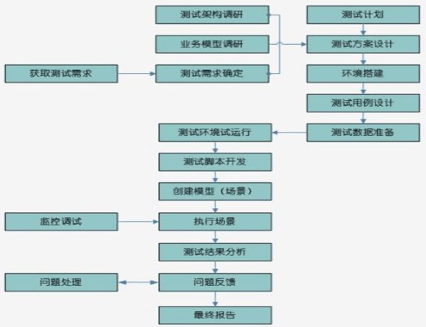
Given a project, how will you conduct performance testing?

Online Fox game server - room configuration wizard - component attribute and basic configuration assignment

Weekly CTF week 1: Amazing tapes

Module 8 - Design message queue MySQL table for storing message data

Verification code is the natural enemy of automation? Let's see how Ali P7 solved it
![[project training] wechat official account to obtain user openid](/img/54/0a77e4441ee87e6ff04f3f07baa965.png)
[project training] wechat official account to obtain user openid
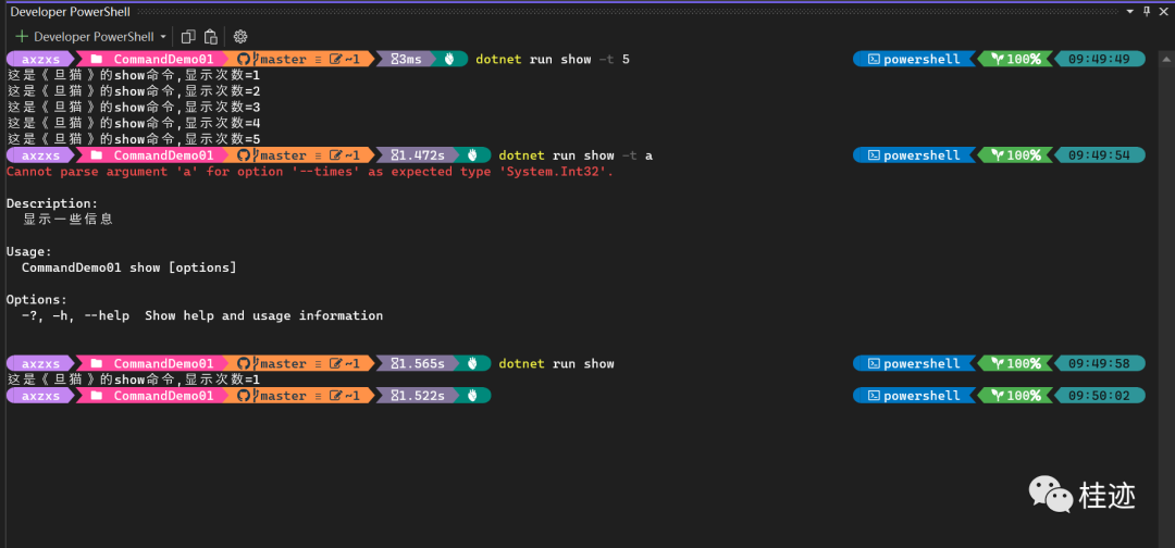
System. Commandline option

Jvm: thread context classloader

How to guarantee industrial control safety: system reinforcement
随机推荐
Given a project, how will you conduct performance testing?
State Administration of market supervision and state Internet Information Office: carry out data security management certification
2022-06-11: note that in this document, graph is not the meaning of adjacency matrix, but a bipartite graph. In the adjacency matrix with length N, there are n points. Matrix[i][j] represents the dist
Lambda创建流
jmeter 性能测试用 csv,这个坑有些扯蛋
Explain asynchronous tasks in detail: the task of function calculation triggers de duplication
System. Commandline option
Image retrieval based on cross modal AI model
Markov networks and conditional random fields
How can functional tests be quickly advanced in one month? It is not a problem to clarify these two steps
C language preprocessing instructions - learning 21
be based on. NETCORE development blog project starblog - (11) access statistics
I worked as a software testing engineer in a large factory and wrote "one day's complete workflow"
市场监管总局、国家网信办:开展数据安全管理认证工作
Interviewer: do you understand redis' shared object pool?
Comparison of OpenCV basic codes of ros2 foxy~galactic~humble
Elegant throttling / de buffeting decorator under LAYA
100 deep learning cases | day 41: speech recognition - pytorch implementation
Forecast report on market demand and future prospect of cvtf industry of China's continuously variable transmission oil
One article to show you how to understand the harmonyos application on the shelves