100 deep learning cases | day 41: speech recognition - pytorch implementation

My environment ：

• Language environment ：Python3.8
• compiler ：Jupyter Lab
• Deep learning environment ：
  • torch==1.10.0+cu113
  • torchvision==0.11.1+cu113
• Creation platform ： Polar chain AI cloud
• Creating tutorials ： Operation manual

In depth learning environment configuration tutorial ： Introduction to Xiaobai, deep learning | Fourth articles ： To configure PyTorch Environmental Science

Previous highlights

1. Deep learning 100 example | The first 1 example ： Cat and dog recognition - PyTorch Realization
2. Deep learning 100 example | The first 2 example ： Facial expression recognition - PyTorch Realization
3. Deep learning 100 example | The first 3 God ： Traffic sign recognition - PyTorch Realization
4. Deep learning 100 example | The first 4 example ： Fruit recognition - PyTorch Realization

• From column ：《 Deep learning 100 example 》Pytorch edition
• Mirror column ：《 Deep learning 100 example 》TensorFlow edition

Our code flow chart is as follows ：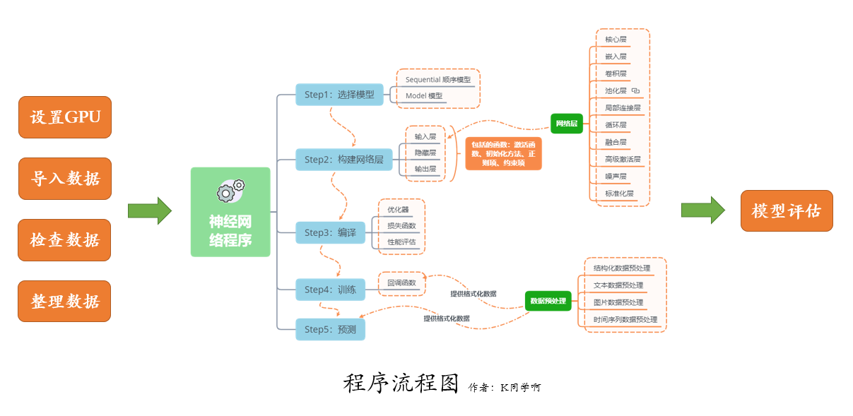

One 、 Import data

I will use torchaudio To download SpeechCommands Data sets , It was recorded by different people 35 It's a command Voice data sets . In this dataset , All the audio files are about 1 Seconds long （ about 16000 Time frame length ）.

The actual loading and formatting steps occur when accessing data points ,torchaudio Responsible for converting audio files into tensors . If you want to load audio files directly , have access to torchaudio.load(). It returns a tuple , It contains the newly created tensor and the sampling frequency of the audio file （SpeechCommands by 16kHz）.

import torch
import torch.nn as nn
import torch.nn.functional as F
import torch.optim as optim
import torchaudio
import matplotlib.pyplot as plt
import IPython.display as ipd
from tqdm import tqdm

Let's check CUDA GPU Is it available and choose our equipment . stay GPU Running the network on will greatly reduce training / Test run time .

device = torch.device("cuda" if torch.cuda.is_available() else "cpu")
print(device)

cuda

1. Download data

from torchaudio.datasets import SPEECHCOMMANDS
import os

class SubsetSC(SPEECHCOMMANDS):
    def __init__(self, subset: str = None):
        super().__init__("./", download=True)

        def load_list(filename):
            filepath = os.path.join(self._path, filename)
            with open(filepath) as fileobj:
                return [os.path.normpath(os.path.join(self._path, line.strip())) for line in fileobj]

        if subset == "validation":
            self._walker = load_list("validation_list.txt")
        elif subset == "testing":
            self._walker = load_list("testing_list.txt")
        elif subset == "training":
            excludes = load_list("validation_list.txt") + load_list("testing_list.txt")
            excludes = set(excludes)
            self._walker = [w for w in self._walker if w not in excludes]

#  Divide training set and test set 
train_set = SubsetSC("training")
test_set  = SubsetSC("testing")

waveform, sample_rate, label, speaker_id, utterance_number = train_set[0]

2. Data presentation

SpeechCommands The data points in the data set are determined by the waveform （ sound signal ）、 Sampling rate 、 word （ label ）、 The speaker ID、 A tuple of words .

print("Shape of waveform: {}".format(waveform.size()))
print("Sample rate of waveform: {}".format(sample_rate))

plt.plot(waveform.t().numpy());

Shape of waveform: torch.Size([1, 16000])
Sample rate of waveform: 16000

labels = sorted(list(set(datapoint[2] for datapoint in train_set)))
print(labels)

['backward', 'bed', 'bird', 'cat', 'dog', 'down', 'eight', 'five', 'follow', 'forward', 'four', 'go', 'happy', 'house', 'learn', 'left', 'marvin', 'nine', 'no', 'off', 'on', 'one', 'right', 'seven', 'sheila', 'six', 'stop', 'three', 'tree', 'two', 'up', 'visual', 'wow', 'yes', 'zero']

35 The audio tags are commands spoken by the user

waveform_first, *_ = train_set[0]
ipd.Audio(waveform_first.numpy(), rate=sample_rate)

waveform_second, *_ = train_set[1]
ipd.Audio(waveform_second.numpy(), rate=sample_rate)

waveform_last, *_ = train_set[-1]
ipd.Audio(waveform_last.numpy(), rate=sample_rate)

Two 、 Data preparation

1. Format data

For waveforms , We down sample the audio to speed up processing , Without losing too much classification ability .

new_sample_rate = 8000

transform   = torchaudio.transforms.Resample(orig_freq=sample_rate, new_freq=new_sample_rate)
transformed = transform(waveform)

ipd.Audio(transformed.numpy(), rate=new_sample_rate)

We use the index in the tag list to encode each word .

2. Encoding and restoration of labels

def label_to_index(word):
    # Return the position of the word in labels
    return torch.tensor(labels.index(word))

def index_to_label(index):
    # Return the word corresponding to the index in labels
    # This is the inverse of label_to_index
    return labels[index]

word_start = "yes"
index = label_to_index(word_start)
word_recovered = index_to_label(index)

print(word_start, "-->", index, "-->", word_recovered)

yes --> tensor(33) --> yes

3. Build a data loader

def pad_sequence(batch):
    # Make all tensor in a batch the same length by padding with zeros
    batch = [item.t() for item in batch] #  take Tensor To transpose 
    #  use 0 Fill the tensor to equal length ,.pad_sequence() For usage, please refer to ：https://blog.csdn.net/qq_38251616/article/details/125222012
    batch = torch.nn.utils.rnn.pad_sequence(batch, batch_first=True, padding_value=0.)
    return batch.permute(0, 2, 1)

def collate_fn(batch):
    # A data tuple has the form:
    # waveform, sample_rate, label, speaker_id, utterance_number
    tensors, targets = [], []
    # Gather in lists, and encode labels as indices
    for waveform, _, label, *_ in batch:
        tensors += [waveform]
        targets += [label_to_index(label)]

    # Group the list of tensors into a batched tensor
    tensors = pad_sequence(tensors)
    targets = torch.stack(targets)
    return tensors, targets

batch_size = 256

if device == "cuda":
    num_workers = 1
    pin_memory = True
else:
    num_workers = 0
    pin_memory = False

#  About torch.utils.data.DataLoader() Students whose usage is not clear , You can refer to the article ：
# https://blog.csdn.net/qq_38251616/article/details/125221503
train_loader = torch.utils.data.DataLoader(
    train_set,
    batch_size=batch_size,
    shuffle=True,
    collate_fn=collate_fn,
    num_workers=num_workers,
    pin_memory=pin_memory,
)
test_loader = torch.utils.data.DataLoader(
    test_set,
    batch_size=batch_size,
    shuffle=False,
    drop_last=False,
    collate_fn=collate_fn,
    num_workers=num_workers,
    pin_memory=pin_memory,
)

for X, y in test_loader:
    print("Shape of X [N, C, H, W]: ", X.shape)
    print("Shape of y: ", y.shape, y.dtype)
    break

Shape of X [N, C, H, W]:  torch.Size([256, 1, 16000])
Shape of y:  torch.Size([256]) torch.int64

3、 ... and 、 Build the model

In this tutorial , We will use convolutional neural network to process the original audio data . More advanced conversion is usually applied to audio data , but CNN It can be used to process raw data accurately . The specific architecture is modeled on the M5 Network architecture . An important aspect of the model processing the original audio data is the receptive field of the first layer filter . The first filter length of our model is 80, Therefore, in the process of 8kHz Sampled audio , The feeling field is about 10ms（ stay 4kHz About 20ms）. This size is similar to that often used from 20 Milliseconds to 40 MS receptive field voice processing application .

class M5(nn.Module):
    def __init__(self, n_input=1, n_output=35, stride=16, n_channel=32):
        super().__init__()
        self.conv1 = nn.Conv1d(n_input, n_channel, kernel_size=80, stride=stride)
        self.bn1 = nn.BatchNorm1d(n_channel)
        self.pool1 = nn.MaxPool1d(4)
        self.conv2 = nn.Conv1d(n_channel, n_channel, kernel_size=3)
        self.bn2 = nn.BatchNorm1d(n_channel)
        self.pool2 = nn.MaxPool1d(4)
        self.conv3 = nn.Conv1d(n_channel, 2 * n_channel, kernel_size=3)
        self.bn3 = nn.BatchNorm1d(2 * n_channel)
        self.pool3 = nn.MaxPool1d(4)
        self.conv4 = nn.Conv1d(2 * n_channel, 2 * n_channel, kernel_size=3)
        self.bn4 = nn.BatchNorm1d(2 * n_channel)
        self.pool4 = nn.MaxPool1d(4)
        self.fc1 = nn.Linear(2 * n_channel, n_output)

    def forward(self, x):
        x = self.conv1(x)
        x = F.relu(self.bn1(x))
        x = self.pool1(x)
        x = self.conv2(x)
        x = F.relu(self.bn2(x))
        x = self.pool2(x)
        x = self.conv3(x)
        x = F.relu(self.bn3(x))
        x = self.pool3(x)
        x = self.conv4(x)
        x = F.relu(self.bn4(x))
        x = self.pool4(x)
        x = F.avg_pool1d(x, x.shape[-1])
        x = x.permute(0, 2, 1)
        x = self.fc1(x)
        return F.log_softmax(x, dim=2)

model = M5(n_input=transformed.shape[0], n_output=len(labels))
model.to(device)
print(model)

def count_parameters(model):
    return sum(p.numel() for p in model.parameters() if p.requires_grad)

n = count_parameters(model)
print("Number of parameters: %s" % n)

M5(
  (conv1): Conv1d(1, 32, kernel_size=(80,), stride=(16,))
  (bn1): BatchNorm1d(32, eps=1e-05, momentum=0.1, affine=True, track_running_stats=True)
  (pool1): MaxPool1d(kernel_size=4, stride=4, padding=0, dilation=1, ceil_mode=False)
  (conv2): Conv1d(32, 32, kernel_size=(3,), stride=(1,))
  (bn2): BatchNorm1d(32, eps=1e-05, momentum=0.1, affine=True, track_running_stats=True)
  (pool2): MaxPool1d(kernel_size=4, stride=4, padding=0, dilation=1, ceil_mode=False)
  (conv3): Conv1d(32, 64, kernel_size=(3,), stride=(1,))
  (bn3): BatchNorm1d(64, eps=1e-05, momentum=0.1, affine=True, track_running_stats=True)
  (pool3): MaxPool1d(kernel_size=4, stride=4, padding=0, dilation=1, ceil_mode=False)
  (conv4): Conv1d(64, 64, kernel_size=(3,), stride=(1,))
  (bn4): BatchNorm1d(64, eps=1e-05, momentum=0.1, affine=True, track_running_stats=True)
  (pool4): MaxPool1d(kernel_size=4, stride=4, padding=0, dilation=1, ceil_mode=False)
  (fc1): Linear(in_features=64, out_features=35, bias=True)
)
Number of parameters: 26915

We will use the same optimization techniques used in this article , That is, the weight attenuation is set to 0.0001 Of Adam Optimizer . At first , We're going to 0.01 The learning rate of training , but scheduler stay 20 individual epoch After the training period , We will use a Reduce it to 0.001.

optimizer = optim.Adam(model.parameters(), lr=0.01, weight_decay=0.0001)
scheduler = optim.lr_scheduler.StepLR(optimizer, step_size=20, gamma=0.1)  # reduce the learning after 20 epochs by a factor of 10

Four 、 Training models

Now let's define a training function , It inputs our training data into the model and performs the reverse transfer and optimization steps . For training , The loss we will use is negative log likelihood . And then will be in each epoch Then test the network , To see how accuracy changes during training .

#  To speed up code running , The accuracy rate is not calculated during training .
def train(model, epoch, log_interval):
    model.train()
    for batch_idx, (data, target) in enumerate(train_loader):

        data   = data.to(device)
        target = target.to(device)

        # apply transform and model on whole batch directly on device
        data   = transform(data)
        output = model(data)

        #  Calculation  loss
        loss = F.nll_loss(output.squeeze(), target)

        optimizer.zero_grad()
        loss.backward()
        optimizer.step()

        #  Print training progress 
        if batch_idx % log_interval == 0:
            print(f"Train Epoch: {
      epoch} [{
      batch_idx * len(data)}/{
      len(train_loader.dataset)} ({
      100. * batch_idx / len(train_loader):.0f}%)]\tLoss: {
      loss.item():.6f}")

        #  Record  loss
        losses.append(loss.item())

#  Calculate the correct number of predictions 
def number_of_correct(pred, target):
    return pred.squeeze().eq(target).sum().item()

#  Find the most likely tag 
def get_likely_index(tensor):
    return tensor.argmax(dim=-1)

def test(model, epoch):
    model.eval()
    correct = 0
    for data, target in test_loader:

        data = data.to(device)
        target = target.to(device)

        # apply transform and model on whole batch directly on device
        data = transform(data)
        output = model(data)

        pred = get_likely_index(output)
        correct += number_of_correct(pred, target)

    print(f"\nTest Epoch: {
      epoch}\tAccuracy: {
      correct}/{
      len(test_loader.dataset)} ({
      100. * correct / len(test_loader.dataset):.0f}%)\n")

Last , We can train and test the network . We will train online 10 individual epoch, Then reduce the learning rate and train again 10 individual epoch. The network will be in every epoch Then test , To see how accuracy changes during training .

log_interval = 100  #  Every time 100 individual batch Print a workout result 
n_epoch = 2

losses = []

# The transform needs to live on the same device as the model and the data.
transform = transform.to(device)

for epoch in range(1, n_epoch + 1):
    train(model, epoch, log_interval)
    test(model, epoch)
    scheduler.step()

Train Epoch: 1 [0/84843 (0%)]	Loss: 3.655148
Train Epoch: 1 [25600/84843 (30%)]	Loss: 2.012523
Train Epoch: 1 [51200/84843 (60%)]	Loss: 1.584120
Train Epoch: 1 [76800/84843 (90%)]	Loss: 1.249869

Test Epoch: 1	Accuracy: 6962/11005 (63%)

Train Epoch: 2 [0/84843 (0%)]	Loss: 0.964569
Train Epoch: 2 [25600/84843 (30%)]	Loss: 1.161757
Train Epoch: 2 [51200/84843 (60%)]	Loss: 1.007113
Train Epoch: 2 [76800/84843 (90%)]	Loss: 0.843660

Test Epoch: 2	Accuracy: 7219/11005 (66%)

1. During the training loss

plt.plot(losses)
plt.xlabel("Step", fontsize=12)
plt.ylabel("Loss", fontsize=12)
plt.title("Training Loss")
plt.show()

5、 ... and 、 test model

def predict(tensor):
    tensor = tensor.to(device)
    tensor = transform(tensor)
    tensor = model(tensor.unsqueeze(0))
    tensor = get_likely_index(tensor)
    tensor = index_to_label(tensor.squeeze())
    return tensor

waveform, sample_rate, utterance, *_ = train_set[-1]
ipd.Audio(waveform.numpy(), rate=sample_rate)

print(f" True value : {
      utterance}.  Predictive value : {
      predict(waveform)}.")

 True value : zero.  Predictive value : zero.

for i, (waveform, sample_rate, utterance, *_) in enumerate(test_set):
    output = predict(waveform)
    if output != utterance:
        ipd.Audio(waveform.numpy(), rate=sample_rate)
        print(f"Data point #{
      i}.  True value : {
      utterance}.  Predictive value : {
      output}.")
        break
else:
    print("All examples in this dataset were correctly classified!")
    print("In this case, let's just look at the last data point")
    ipd.Audio(waveform.numpy(), rate=sample_rate)
    print(f"Data point #{
      i}.  True value : {
      utterance}.  Predictive value : {
      output}.")

Data point #1.  True value : right.  Predictive value : no.