Yolact paper reading and analysis

YOLACT:Real-time Instance Segmentation

Abstract

This paper presents a simple 、 Full convolution real-time instance segmentation model , stay MS COCO In order to 33.5fps The speed of 29.8mAP, And only in one gpu This is the result of training .
In this paper, instance segmentation is divided into two subtasks ：
(1) Generate a series of prototype masks
(2) Predict the... Of each instance mask coefficient
And then by putting prototype and mask The coefficients are linearly combined to generate instance masks
The author finds that this process does not depend on repooling, Can produce high quality masks also exhibits tem-
poral stability for free（ Show stability ？)
Besides , This paper analyzes prototypes Sudden behavior of , Found that although they are fully-convolutional, But in a way translation variant You can do it yourself localize
This paper also presents a comparison of NMS Faster Fast NMS

introduction

What is required to create a real-time instance segmentation algorithm ？
Over the past few years , Great progress has been made in the field of instance segmentation , Part of the reason is to take advantage of the powerful parallelism in the established target detection field . The most advanced instance segmentation algorithm ( Such as Mask RCNN and FCIS) Directly based on the development of target detection ( Such as Faster R-CNN and R-FCN). These methods focus on performance rather than speed , A real-time target detector that leads to the lack of real-time instance segmentation ( Such as SSD and YOLO). The goal of this article is to use a fast 、 Single stage (one-stage) To fill this gap , It's like SSD and YOLO It fills the blank of target detection .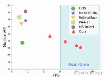

**coco Speed performance comparison of various instance segmentation methods on **

But instance segmentation is much more difficult than object detection , similar YOLO and SSD Of one-stage The target detector can simply remove the second stage and compensate for the performance loss in other ways to speed up the existing two-stage detector ( Such as Faster R-CNN). But the same method is not easy to extend to the field of instance segmentation .SOTA Whether the two-stage instance segmentation algorithm depends on feature localization( Feature location ) To produce mask. That is to say, these methods are used in some bounding box areas “ Heavy pooling (repool)”( Use RoI-pool/align Other methods )
, Then put these localized features Input to mask In the predictor . This method is essentially sequential , So it's hard to accelerate . There are also some things like FCIS Such a method of performing these steps in parallel , But they need to be in localization After a lot of post-processing , So it's far from real-time .
In order to solve the above problems , Put forward YOLACT, A real-time instance segmentation framework , It abandons explicit localization step .YOLACT Split the instance into two parallel tasks ：
(1) Generate... On the entire image non-local prototype masks Dictionary
(2) Predict a set of linear combination coefficients for each instance
Then generate a complete image instance from these two components. Segmentation is simple ： For each instance , Use the corresponding prediction coefficient to linearly combine prototypes, Then crop out the predicted bounding box . This paper shows how to segment , The Internet has learned how to localize example masks, On the vision 、 Examples that are spatially and semantically similar are prototypes Show a difference .
Besides , because prototype masks The number of is independent of the number of categories ( Such as ： Categories can be compared to prototypes many ).YOLACT Learned a distributed representation , Each of these instances is shared across categories prototypes Combine and divide . This distributed representation is in prototype There are interesting sudden behaviors in space : some prototypes Space division of image 、 Some positioning examples 、 Some detection instance contours 、 Some coding position sensitive patterns ( Similar to FCIS Hard code those obtained by a location sensitive module in ), Most of them are combinations of these tasks .
This approach has several practical advantages . First and foremost ： Fast ： Because of its parallel structure and extremely lightweight assembly process ,YOLACT Only a small amount of computing overhead is added to the primary trunk detector , Even in use ResNet101 when , It's also easy to achieve 30fps Per second ; In fact, the whole mask The evaluation of the branch only needs 5ms. second ,masks It's of high quality ： because masks The whole range of image space is used , Not because repooling Lose any quality , our masks The mass of large objects is significantly higher than that of other methods ( Pictured 7). Last , It is general ： Generate prototypes and masks The idea of coefficients can be applied to any modern target detector .
The main contribution of this paper is ： First real time (>30fps) Instance segmentation algorithm , And in challenging MS COCO Competitive results were obtained on the data set ( See the picture 1). Besides , This paper analyzes YOLACT Of prototypes Sudden behavior of , And provide experiments to study in different backbone architectures 、prototypes The tradeoff between speed and performance obtained under quantity and image resolution . This paper also presents a new Fast NMS Method , Than traditional NMS fast 12ms, The performance loss is negligible .
YOLACT Code for ：(https://github.com/dbolya/yolact)

Related work

Instance segmentation

Because of its importance , People have done a lot of research to improve the accuracy of instance segmentation .Mask-RCNN It is a typical two-stage instance segmentation method ： First, candidate regions of interest are generated (region-of-interests,ROI), And then in the second stage, we'll do some research on these ROIs Classification and segmentation . The follow-up work tries to enrich FPN Characteristic or solution mask The incompatibility between the confidence score and its positioning accuracy to improve its accuracy . These two-phase approaches require re-pooling Every ROI Characteristics of , And deal with them through subsequent calculations , This makes it impossible for them to get real-time speed (30fps), Even if the picture size is reduced ( See the picture 2c).
The single-stage instance segmentation method generates a location sensitive graph (position sensitive maps), Through location sensitive pooling (position-sensitive pooling) Assemble into the final masks, Or combined with semantic segmentation logits And direction prediction logits. Although conceptually faster than the two-phase approach , But it still needs repooling Or other important calculations ( Such as mask voting). This severely limits their speed , Make them not real-time . by comparison , Our assembly steps are much lighter ( Just a linear combination ), And can be implemented as a gpu Accelerated matrix - Matrix multiplication , It makes our method very fast .
Last , Some methods start with semantic segmentation , Then carry out boundary detection , Pixel clustering or learning embedding to form instances masks. Again , These methods have multiple stages and \ Or involve expensive clustering processes , This limits their viability for real-time applications .

Real time instance segmentation

Although there are real-time object detection and semantic segmentation , But few people pay attention to real-time instance segmentation .《Straight to Shapes》 and 《Box2Pix》 Instance segmentation can be performed in real time (《Straight to Shapes》 stay Pascal SBD 2012 The number of frames on is 30fps, stay Cityscapes The number of frames on is 10.9fps,《Box2Pix》 stay KITTI The number of frames on is 35fps), But they are far less accurate than modern benchmarks . in fact ,Mask R-CNN It is still one of the fastest instance segmentation methods on semantically challenging data sets , Such as COCO( stay 550 Pixel image up to 13.5fps, See table 2c).

Prototypes

Learning prototypes ( also called aka vocabulary or code-book) stay cv The field has been extensively studied . Classic includes text (textons) And visual words (visual words), It is improved by sparsity and local prior . Others have designed target detection prototypes. Although relevant , These jobs use prototypes To represent a feature , And we use them to assemble masks Split instances . Besides , We learn prototypes Is specific to each image , Instead of the global shared by the entire dataset prototypes.

3.YOLACT

chart 2：YOLACT framework ： Blue / Yellow indicates prototypes Medium low / High value , Grey nodes indicate untrained functions , In this case k=4, Use ResNet101+FPN stay RetinaNet This framework is established on the basis of

Our goal is like mask R-CNN and Faster R-CNN equally , Add one to the existing single-stage target detection model mask Branch , But there is no clear feature location step ( Such as characteristics repooling). To do this , We decompose the complex task of instance segmentation into two simpler tasks 、 Parallel tasks , They can be assembled into the final masks. The first branch uses FCN Generate an image size “prototype masks”, They do not depend on any one instance . Second add an extra head Go to the target detection branch to predict the "mask coefficient " vector , These anchors are prototype The existence of an instance is encoded in the space . Finally, for each existing in NMS Example , Use the work of linearly combining the two branches to construct a mask.

Rationale

This paper uses this method to segment instances , Mainly because masks It is continuous in space , That is, pixels close to each other may be part of an instance . Although the convolution (conv) It is natural to take advantage of this consistency , But the full connectivity layer (fc) But not . This raises a problem , Because the single-stage target detector generates classes and for each anchor box Coefficient as fc Layer output . The two-stage approach is as follows Mask R-CNN By using localization step ( Such as RoI-Align) To solve this problem , It preserves the spatial consistency of features , Also run maks As a conv Layer output . However , Doing so requires a large part of the model to wait for the first phase RPN To carry out localization The candidate , Resulting in a significant loss of speed .
therefore , This paper divides the problem into two parallel parts , Make use of those who are good at generating semantic vectors fc Layers and those who are good at generating spatial coherence masks Of conv Layers are generated separately “mask coefficient ” and “prototype masks”. And then because of prototypes and mask The coefficient can be calculated separately , The computational overhead relative to the backbone detector mainly comes from the assembly steps , This enables a single matrix multiplication . by this means , While maintaining the spatial consistency of feature space , It is still single-stage 、 fast

3.1 prototype Generation

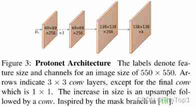
prototype Generate branch (protonet) Predict a set of... For the entire image k individual prototype masks. We will protonet Implemented as a FCN, Its last layer has k Channels ( Every prototype There's a tunnel ), And connect it to a backbone feature layer ( See the picture 3). Although this expression is similar to standard semantic segmentation , But the difference is that we are prototypes There is no obvious loss on the . contrary , For these prototypes All supervision comes from the final masks Loss .
We noticed two important design choices ： From deeper backbone features protonet Can produce more robust masks, Higher resolution prototypes Can produce higher quality masks And better performance on smaller targets . therefore , We use FPN Because of its largest feature layer ( In the example P3, See the picture 2) Is the deepest . Then we sample it to a quarter of the size of the input image to improve the performance on small targets .
Last , We found that protonet The unbounded output of is very important , Because this allows the network to be prototypes Produce huge 、 Powerful activation , Make it very believable ( Such as obvious background ). So we can choose to have ReLU Or no non-linear protonet. We can use ReLU Get more explicable prototypes

3.2 Mask Coeffcients

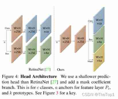
Typical anchor based target detectors in their predictions head There are two branches in ： A branch prediction c Category confidence , Another prediction 4 individual bounding box Return to . about mask Coefficient prediction , We just need to add a third branch prediction in parallel k individual mask coefficient , Every prototype Corresponding to one . therefore , Not every anchor produces 4+c A coefficient of , But produce 4+c+k A coefficient of .
And then for nonlinearity , We found that from the final mask Subtract from prototypes It's important . So we will tanh Applied to the k mask coefficient , Thus, a more stable output can be produced without nonlinearity . The relevance of this design is shown in the figure 2 Shown , Because if you don't consider subtraction , Two mask Are not constructable .

3.3 Mask Assembly

To generate instances masks, We will prototype Branches and mask The work of the coefficient branch is combined , Use the linear combination of the former and the latter as the coefficient . And then through a sigmoid Nonlinear to produce the final masks. Use a single matrix to multiply and sigmoid These operations can be effectively implemented ：

among P yes prototype masks Of hwk matrix ,C Is in NMS And the score threshold n An example of mask One of the coefficients n*k matrix . Other more complex combination steps are also possible ; However, we keep it simple through a basic linear combination ( And fast )

losses

Use three kinds of losses to train the model ： Classified loss $L_{cls}$,box Return to loss $L_{box}$ and mask Loss $L_{mask}$, The weights are 1,1.5 and 6.125.$L_{cls}$ and $L_{box}$ Definition and SSD In the same . And then to calculate mask Loss , We just need to put it together masks M and ground truth masks The binary cross entropy at pixel level is calculated $L_{mask}=BCE(M,M_{gt})$

Cropping Masks

In the process of evaluation , Use predicted bounding box Cut out the final masks. Use... In training ground truth bounding box, take $L_{mask}$ Divide ground truth bounding box Area to preserve prototypes Small targets in .

3.4 Emergent Behavior

Our approach is amazing , Because it is generally about FCNs The general consensus is that ：FCNs It's translational , So the task needs to be done in 【24】 Add translation variability to . So like FCIS and Mask R-CNN This method explicitly adds translational variability , Whether through directional maps And location sensitive repooling, Or will mask Branch to the second stage , So it doesn't have to deal with localizing example . In our approach , The only way to add translational variability is with predictive bounding box Intercept the final masks. then , We found that our method is also applicable to medium and large targets that do not intercept , So this is not the result of interception . contrary ,YOLACT Learned how to pass prototypes The different activation functions in localize example .
Understand how this is achieved , First of all, notice that there is no padding Of FCN in , chart 5 Medium solid red image ( Images a) Of prototype activations It's actually impossible . Because convolution is output to a single pixel , If its input is the same anywhere in the image , So in conv The result is the same everywhere in the output . On the other hand , image ResNet Such a modern FCNs Consistent edges in padding The network can judge how far the pixel is from the image edge . conceptually , One way it can do this is to fill multiple layers in sequence 0 Spread from the edge to the center ( It's similar to using [1,0] The core of ). It means ResNet The instance itself is translational variable , Our method makes a lot of use of this feature ( Images b and c It shows obvious translational variability ).
We observed many prototypes In some of the images " Partition " Is activated on . in other words , They are only activated on the target on one side of the boundary that is implicitly learned . In the figure 5 in , Prototype 1-3 This is the case . By combining these partition maps , The network can distinguish different semantic classes ( Even overlap ) example , For example, in figure d in , By getting from prototype2 Subtract from prototype3 You can separate the green umbrella from the red umbrella .
Besides , As learning object ,prototypes Is compressible . That is to say if protonet Will be multiple prototypes The functions of , that mask The coefficient branch can learn which conditions and functions are required . for example , In the figure 5 in ,prototype2 Is a partition prototype , But it will also be very strong in the example in the lower left corner .prototype3 similarly , But for the example on the right . This also explains why in practice , Even when used as low as k=32 Of prototypes( See table 2b), The performance of the model will not be reduced . On the other hand , increase k It is likely to be invalid , Because the prediction coefficient is very difficult . Because of the properties of linear combination , If the network produces a large error in a parameter , Generated mask It can disappear or cause the loss of other targets . therefore , The network must act as a balance to produce the correct coefficients , And add more prototypes Will make it difficult . actually , We found that , For the higher k value , The network only adds redundancy prototypes, The change at the edge level is small , Slightly increased $A{P}_{95}$, But not many other changes .

Backbone Detector

For trunk detectors , We prioritize speed and feature richness , Because these predictions prototypes And the coefficient is a difficult job , Good characteristics are needed to do well . Therefore, our trunk detectors strictly comply with RetinaNet, And emphasize speed .

YOLACT Detector

We use the FPN Of ResNet-101 As the default feature trunk , The basic image size is 550*550. We do not keep the aspect ratio , To obtain a consistent evaluation time for each image . image RetinaNet equally , We do not produce $P_2$ and $P_6$ and $P_7$ To modify the FPN, As from $P_5$( instead of $C_5$) The beginning of the continuum 3x3, In steps of 2 Of conv layer , And set on each floor 3 The length width ratio is [1,1/2,2] The anchor of .$P_3$ Our anchors are 24 Square area of pixels , Each subsequent layer is twice the area of the previous layer ( Area is [24,48,96,192,384]). For connecting to each $P_i$ The forecast head, We have one by 3 Shared by branches 3x3 Of conv, Any branch gets its own in parallel 3x3conv. And RetinaNet comparison , Our prediction head Design ( Pictured 4) Lighter , faster . We will $smooth{L}_1$loss Apply to training box Return to , And with SSD The same way for box Regression coordinates for coding . For training class prediction , We use softmax Cross entropy c A positive label and 1 A background tag , Use one 3：1( negative ： just ) Proportional OHEM Select training samples . therefore , And RetinaNet The difference is that we don't use focal loss, We found that this did not apply in our case .
Through these design choices , We found that with the same picture size , This trunk is better than using ResNet Of SSD Better performance , Faster .

5.Other Improvements

We also discussed other improvements , These improvements either increase the speed , But it has little impact on performance , Or the performance is improved , Without loss of speed .

Fast NMS

Generate... For each anchor bounding box Regression coefficient and category confidence , Like most target detectors , We execute NMS To suppress duplicate detection . In many previous jobs ,NMS It's done in order . in other words , For each of the data sets c class , Sort the detected boxes in descending confidence order , Then for each test , Delete all items with confidence lower than it 、IoU Overlap boxes larger than a certain threshold . Although this method 5fps The speed is fast enough , But it is gain 30fps A big obstacle to ( for example ,5fps when 10ms The improvement of results in 0.26fps Raise , but 30fps when 10ms The improvement of results in 12.9fps The promotion of ).
In order to adjust the tradition NMS The order of , We introduced Fast NMS, This is a NMS A version of , In this version , Each instance can be preserved or discarded in parallel . Do that , We only need to allow deleted detections to suppress other detections , It's in the traditional NMS It's impossible . This relaxation allows us to be completely in line with the standard GPU Accelerated matrix operation NMS.
To carry out Fast NMS, Let's first calculate before n A prediction cnn Pair IoU matrix X, By each c The categories are arranged in descending order of scores .GPU Batch sorting on is easy to obtain , Calculation IoU It's also easy to vectorize . then , If there is any test with a higher score , And accordingly IoU Greater than a certain threshold t, We will delete detection . Let's start with X The lower triangle and diagonal of are set to $0:X_{kij}=0,\forall k,j$, This can be done in a batch triu Execute... In the call , Then take the maximum value of the column

Calculate the maximum in each test IoU Value matrix K. Last use t(t<K) Thresholding the matrix will indicate which tests are reserved for each category .
Because loose ,Fast NMS A little too much is removed boxes The effect of . However , Compared with the sharp increase in speed , The resulting performance loss is negligible （ See table 2a）. In our code base ,Fast NMS Than traditional NMS Of Cython Fast implementation 11.8 millisecond , The performance is only reduced 0.1 mAP. stay Mask R-CNN benchmark suite in ,Fast NMS Than CUDA The tradition of fulfillment NMS fast 15.0 millisecond , The performance loss is only 0.3 mAP

Semantic Segmentation Loss

although Fast NMS Trade a small amount of performance for speed , But there are also ways to improve performance without slowing down . One way is to use modules that were not executed during the test to impose additional losses on the model during training . This effectively increases the richness of features , At the same time, there is no speed loss .
therefore , We only apply semantic segmentation loss during training . Note that we constructed the missing from the instance annotation ground truth, So this does not strictly capture semantic segmentation ( That is, there is no mandatory standard of one class per pixel ). To create predictions during training , We need to put one with c Output channel's 1x1conv The layer is directly connected to the largest in the trunk feature map($P_3$) On . Since each pixel can be assigned to multiple classes , We use sigmoid and c Channels replace softmax and c+1. The weight of this loss is 1, And lead to 0.4 Of mAP promote .

6.Results

We use standard metrics reports MS COCO and Pascal 2012 SBD Instance segmentation results on . about MS COCO, We are train2017 Training , stay val and test-dev On the assessment .

Implementation Details

We use ImageNet The weight of pre training is in a gpu Training batchsize by 8 All models of . We found that this is a sufficient batch size to use batch norm, So we keep the unfrozen pre training batch norm But do not add any bn layer . We use SGD Conduct 800k Iterative training , The initial learning rate is $10^{-3}$, In iteration 280k、600k、700k and 750k Time divided by 10, Use $5\times 10^{-4}$ Weight decay of ,0.9 Momentum and SSD All data enhancements used in . about Pascal, We train 120k Sub iteration , stay 60k and 100k Divide the learning rate . We also multiply the size of the anchor by 4/3, Because goals tend to be bigger .COCO At one Titan Xp Training on the needs 4-6 God ( It depends on the configuration ), stay Pascal The training on 1 God .

Mask Results

Let's start with the table 1 Medium MS COCO Of test-dev Set comparison YOLACT And state-of-the-art methods . Because our main goal is speed , So we compare it with other single model results that do not increase the test time . We reported on a Titan Xp All speeds calculated on , So some of the listed speeds may be faster than those in the original file .
YOLACT-550 Provides highly competitive instance segmentation performance , And the speed is COCO The fastest instance segmentation method before 3.8 times . We also note that , Compared with other methods , There is an interesting difference in the performance of our approach . From us in figure 7 Qualitative findings in , stay 50% Under the overlap threshold ,YOLACT-550 and Mask R-CNN The gap between them is 9.5 AP, And in the 75%IoU Below the threshold , The gap is 6.6 AP. This is related to FCIS The performance of , For example, gap coincident Mask R-CNN comparison (AP Values, respectively 7.5 and 7.6). Besides , At the top (95%) Of IoU threshold , Our performance is better than Mask R-CNN, Respectively 1.6 and 1.3AP.
We are on the table 1 The number of candidate model configurations is reported in . In addition to our basic 550×550 Image size outside the model , We also train 400×400（YOLACT-400） and 700×700（YOLACT-700） Model , The range of the anchor is adjusted accordingly ($s_x=s_{550}/550\ast x$). Reducing the image size can result in significant performance degradation , This shows that instance segmentation naturally requires a larger image . then , As expected , Increasing the image size will significantly reduce the speed , But it also improves performance .
In addition to our basic backbone ResNet-101, We also tested it ResNet-50 and DarkNet-53, To get faster results . If a higher speed is needed , We recommend using ResNet-50 or DarkNet-53, Instead of reducing the image size , Because the performance ratio of these configurations YOLACT-400 Much better , But just a little slower .
Last , We also Pascal 2012 SBD It's good for us ResNet-50 The model was trained and evaluated , As shown in the table 3 Shown .YOLACT Obviously better than that in the report SDB Common methods of performance , At the same time, the speed is also significantly accelerated .

Mask Quality

Because we generated a size of 138x138 In the end mask, And because we create directly from the original features masks( Don't use repooling To transform and shift features ), What we use for big goals masks The quality is obviously higher than Mask R-CNN and FCIS Those of masks. for example , In the figure 7 in ,YOLACT Generates a clear line along the arm boundary mask, and FCIS and Mask R-CNN There is more noise . Besides , Although overall mAP Bad 5.9, But in 95%IoU Below the threshold , Our model achieves 1.6AP, and Mask R-CNN achieve 1.3AP. This shows that repooling It does lead to mask A decline in quality .

Temporal Stability

Although we only use static images for training , Do not apply any temporal smoothing, But what we found was that , Our model produces time stable video masks Than Mask R-CNN Bigger , Latter masks Jitter between frames , Even if the object is stationary . We believe in our masks A more stable , Part of the reason is that they are of higher quality （ Therefore, the error space between frames is smaller ）, But mainly because our model is single-stage . The two-stage method produces masks Highly dependent on regional proposals in the first phase (region proposals). Our approach is different : Even if the model predicts different... Between frames boxes,prototypes And it won't be affected , So as to produce more stable in time masks.

Discussion

Despite our maks With higher quality and better performance , Such as time stability , But the overall performance lags behind the most advanced instance segmentation methods , Although much faster . Most errors are caused by errors in the probe ：misclassification,box-misalignment etc. . However, we have determined that YOLACT Of masks Two typical errors caused by the generation algorithm .

Localization Failure

If there are too many targets in one location in the scene , The network may not be able to prototype Locate each target in . In these cases , The network output will be closer to the future mask The content of , Instead of instance splitting of some targets in the group . For example, in figure 6 The first picture in ( First row, first column ) in , The blue truck under the red plane is not correctly positioned .

Leakage

Our network makes use of mask The condition of being cut after assembly , There is no attempt to suppress noise outside the clipping region . When the bounding box is accurate , This method works well , But when the bounding box is not accurate , Noise may affect the instance mask, Causes some... To occur outside the crop region "leakage". This can also happen when two instances are far away from each other , Because the Internet has learned that it doesn't need localize Distant instances , Clipping will handle this situation . However, if the predicted bounding box is too large ,mask Will also include some remote instances of mask. For example, figure 6( The first 2 Xing di 4 Column ) Shows this leakage, because mask The branch thinks that the three skiers are far enough away from each other without having to separate them .

Understanding the AP Gap

But only localization Failure and leakage Not enough to explain YOLACT The basic model and Mask R-CNN Almost 6 mAP The gap between . in fact , We are COCO The basic model on the test-dev Testing and box mAP(29.8 mask,32.3 box) Only between 2.5mAP The gap between , This means that even with the perfect masks, Our model can only get a little mAP. Besides ,Mask R-CNN Have the same mAP differences (35.7mask,38.2box), This shows that the difference between the two methods lies in the relatively poor performance of our detector , Instead of us generating mask Methods .

A.Appendix

A.1. Box Result

because YOLACT In addition to generating masks Also generated boxes, We can also compare its target detection performance with other target detection methods . Besides , Although our mask Performance is real-time , But we are using YOLACT As a target detector, there is no need to generate masks. therefore ,YOACT Generate at run time boxes Time to run build masks It's faster , In the table 4 in , We compare our performance and speed with YOLOv3 The various versions of .
therefore , We can get the same results as YOLOv3 Similar test results , At the same time, do not use YOLOv2 and YOLOv3 Any other improvements in , Such as multi-scale training,optimized anchor boxes, cell-based regression encoding, and objectness score. Because in our observations , The improvement of detection performance mainly comes from the use of FPN And use masks Training ( Both are related to YOLO The improvements made have intersections ), So it is very likely that YOLO and YOLACT Combine , Create a better detector .
Besides , These results show that , our mask The branch only needs... In total 6 Milliseconds to evaluate , It shows us that mask How small the calculation is .

A.2. More Qualitative Results

chart 6 Shows many examples of adjacent people and vehicles , But there are not many examples of other categories . To further support YOLACT It's not just about semantic segmentation , We are in the picture 8 More qualitative results are included in , These results are for images with adjacent instances of the same class .
for example , In an image with two elephants （ chart 8 The first 2 That's ok , The first 2 Column ）, Although the two instance boxes overlap each other , But their masks The instances are clearly separated . Zebras （ The first 4 That's ok , The first 2 Column ） And birds （ The first 5 That's ok , The first 1 Column ） This is also clearly demonstrated by the example of .
Please note that , For some of these images ,box Not completely from mask Cut it down , This is because for speed reasons ( And the model is trained in this way ), We use prototype Resolution clipping mask( That is, one fourth of the image resolution ), There are... In each direction 1px Fill of . On the other hand , Corresponding box Display at original image resolution , of no avail padding.