Mathematical modeling of war preparation 30 regression analysis 2

Catalog

One 、 The mission of regression analysis

Two 、 Classification of regression analysis

3、 ... and 、 Data classification and processing methods

Four 、 Interpretation of regression coefficients

5、 ... and 、 Handling of special variables

6、 ... and 、 Regression analysis case

---

One 、 The mission of regression analysis

The three missions of regression analysis are as follows ： First of all 、 Identify important variables , You can use stepwise regression ; second , Determine the direction of correlation , Positive correlation or negative correlation ; Third , Estimate the weight , Calculate the regression coefficient .

Two 、 Classification of regression analysis

The regression analysis created is divided into the following categories , We mainly consider linear regression , Nonlinearity can also be learned .

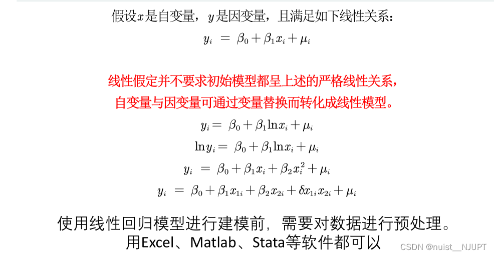
Of course, the said linearity is not strictly linear , The following can be converted to linear by variable substitution , We can all understand it as linear , In fact, strictly speaking, it is nonlinear to linear .

3、 ... and 、 Data classification and processing methods

We need to consider the classification of data , Generally for cross-sectional data , We use regression analysis ;

Cross section data ： Data of different objects collected at a certain point in time , for example ： Provinces across the country 2018 year GDP The data of

time series data ： Data obtained by continuous observation of the same object at different times , for example ： Over the years, China GDP

A data resource that combines cross-sectional data with time series data , for example ：2008‐2018 year , Provinces in China GDP The data of .

Four 、 Interpretation of regression coefficients

We make a point estimate of the regression equation , After calculating the regression coefficient , The regression coefficient needs to be explained , In fact, it is to explain the relationship between independent variables and dependent variables , In fact, you will find that the number of independent variables is different , It has a great influence on the regression coefficient , That is to say, for the core explanatory variable, we need to treat it as an independent variable , We need to make the core explanatory variable independent of the perturbation term

We let the error term and all the arguments x It's not relevant , Make the model exogenous , If relevant , There will be endogeneity , The estimated value of regression coefficient is inaccurate . 

We want to make the regression model non endogenous , It is generally required that the explanatory variable is independent of the disturbance term , But there are many explanatory variables , We only consider that the price core explanatory variable is independent of the disturbance term , It is not necessary to consider all explanatory variables . 

Sometimes , We can take logarithms of independent variables and dependent variables , Taking logarithms has three advantages ,

5、 ... and 、 Handling of special variables

For quantitative variables , Generally, it can be directly regressed , For qualitative variables , Such as gender , regional , There are no specific numbers , What do we need to do , This needs to consider the problem of dummy variables .

If we study the impact of gender on wages , As shown below ：

  We need to explain the dummy variables , The coefficient can be understood as the difference , That is, when other independent variables are the same , On average , Women earn less per hour than men 1.81 dollar . 

6、 ... and 、 Regression analysis case

The following regression analysis case is to explain the regression model , A general regression equation is used to explain or predict , This is mainly used to explain , In addition, this question uses stata Software implementation .

  First of all, will excel Data import in stata, As follows ：

Descriptive statistics are generally required before regression , It is to describe and count the data information in the table , As follows ： We first divide the data in the topic into quantitative data and qualitative data , As follows ：

For quantitative data ,stata The descriptive statistical method of is as follows , Namely summarize The form of adding variables .
   For qualitative variables , We want to get the frequency distribution table of the corresponding variables , And generate the corresponding virtual variable , The details are as follows , In the command window , Use tabulate that will do .

Now we need to establish the regression equation , And carry out regression analysis ,stata The regression statement for is as follows ：,p Less than 0.05, Rejection of null hypothesis , It is considered that the regression model is established .coef It's the regression coefficient .

Direct use of quantitative data regress Statement for regression , For qualitative statements , We need to add a dummy variable after , And then go back , So the first question is solved , As follows ：

Let's take a look ,p About equal to 0, You can reject the original hypothesis , It shows that the regression equation is significant as a whole , You will find that only two variables are significant , So we use two independent variables to explain the evaluation quantity . 

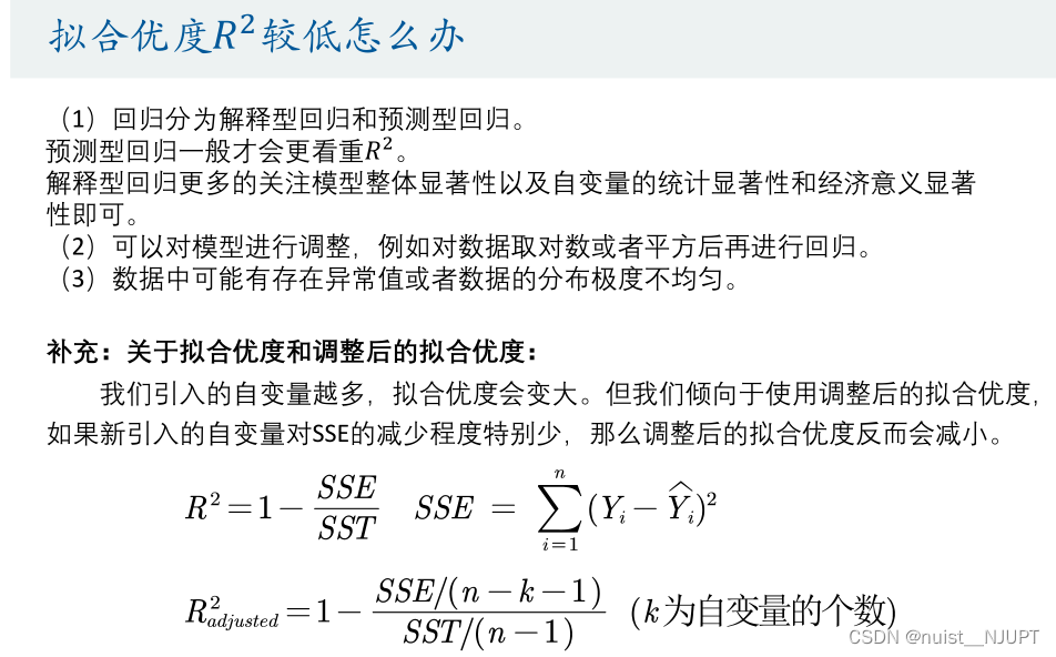
  Regression analysis , We usually need to consider the goodness of fit problem , Generally speaking, for explanatory regression , Less emphasis on goodness of fit , Predictive regression pays more attention to goodness of fit . For regression model , We prefer to use the adjusted goodness of fit .

For the first 2 ask , Study the important factors of evaluation quantity , We can use standardized regression , After standardizing the original data , The regression equation is established with the standardized data , The greater the absolute value of the regression coefficient , It means that the greater the impact on the evaluation quantity .

For the perturbation term , It is necessary to satisfy the two conditions of CO variance and no autocorrelation , Therefore, heteroscedasticity test is required .

Homovariance ： The variance of the perturbation term is the same , The correlation of any two perturbation terms is 0.

  If the perturbation term has heteroscedasticity , The hypothesis test cannot be used , And the ordinary least squares is no longer the optimal linear unbiased estimator .

  We can use stata To draw a scatter chart , It is speculated whether there is Heteroscedasticity in the perturbation term . When the fitting value is very small , There is no fluctuation in the data , When the data is large , The data fluctuates greatly . When the group purchase price is very small , Data is volatile , Words behind , Small fluctuation , Therefore, it is speculated that there is heteroscedasticity .

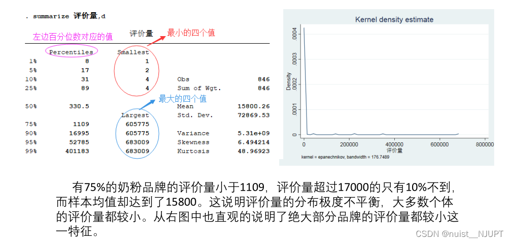
  In fact, we find that the fitting value is negative , You can plot the probability density function , It can be found that the distribution of evaluation quantity is uneven , Use summarize The instruction can get the descriptive statistics of the evaluation quantity ; The non-uniform distribution of evaluation quantity leads to small goodness of fit , The fitting value is negative , The specific analysis is as follows ：

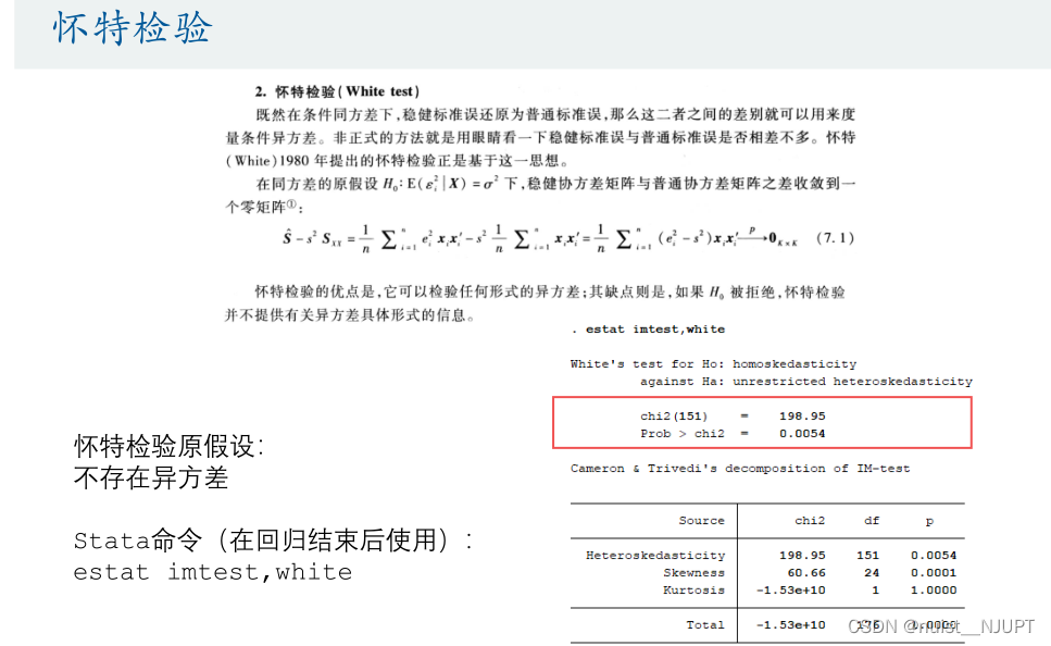
  The heteroscedasticity test of graphs is rough , We use the hypothesis test of heteroscedasticity , There are two main kinds of ：BP Test and white test . Let's see ：

We found that P Less than 0.05, Rejection of null hypothesis , It indicates that there is heteroscedasticity .

  Let's take a look at the white test , Rejection of null hypothesis , There is heteroscedasticity , Anyway , There is no heteroscedasticity .

  If heteroscedasticity occurs , We use the 1 There are three ways to solve the heteroscedasticity problem ,

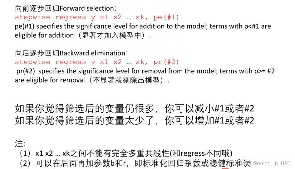
For possible multicollinearity problems , We usually use stepwise regression to solve , If the explanatory variables are linearly correlated , Then there is a multicollinearity problem , Multi industry collinearity will lead to unreasonable coefficient estimation , Even the opposite of the expected symbols .

We usually use the variance expansion factor to test the multicollinearity of heavy industry , Think VIF Greater than 10, It shows that the regression equation has serious multicollinearity .

  For multicollinearity problems , We generally adopt the following methods , If you use an equation to predict , Then the multicollinearity problem does not need to be considered . In addition, although the relationship between the specific regression coefficient , However, multicollinearity does not affect the significance of the variables concerned , You don't need to think about it , Stepwise regression is considered only if multicollinearity affects the significance of the variable under consideration .

For stepwise regression , We can consider using previous stepwise regression or backward stepwise regression , As follows ：

stata The statement to implement stepwise regression is as follows ：

  The results of two stepwise regression may be different , And it should be noted that the stepwise regression needs to propose fully multicollinearity variables in advance , Otherwise, an error will be reported , Ordinary regression , There is no need to manually eliminate ,stata Will be automatically eliminated .

stata The source code is shown below , In addition to regression , Residual analysis and heteroscedasticity test are also carried out .

clear
//  Clear the screen   and  matlab Of clc similar 
cls 
//  Import data （ In fact, we pasted it directly on the interface , It is more convenient for us to import with the mouse click interface   Please delete this clause and then copy it into the thesis , If the judge teacher sees it, he will know that you didn't write it ）
// import excel "C:\Users\hc_lzp\Desktop\ Mathematical modeling video recording \ The first 7 speak . Multiple regression analysis \ Code and example data \ Milk powder data explained in class .xlsx", sheet("Sheet1") firstrow
 import excel "C:\Users\nuist__NJUPT\Desktop\ Digital analog algorithm source code - Wang Guodong \ regression analysis \ Milk powder data explained in class .xlsx", sheet("Sheet1") firstrow
//  Descriptive statistics of quantitative variables 
summarize  The group purchase price is yuan   Evaluation quantity   Gross weight of goods kg
//  Frequency distribution of qualitative variables , And get the virtual variable starting with the corresponding letter 
tabulate  formula ,gen(A)
tabulate  Milk origin  ,gen(B)
tabulate  Domestic or imported  ,gen(C)
tabulate  The applicable age is  ,gen(D)
tabulate  Packaging unit  ,gen(E)
tabulate  classification  ,gen(F)
tabulate  Dan  ,gen(G)
//  Let's go back 
regress  Evaluation quantity   The group purchase price is yuan   Gross weight of goods kg
//  The following statement can help us save the regression results in Word In the document 
//  Before using, you need to run the following code to install the function package （ After running once, you can comment out ）
//ssc install reg2docx, all replace
//  If the installation appears connection timed out Error of , You can try to switch to mobile hotspot networking , If the mobile phone hotspot cannot be downloaded , Don't use this command , You can make a regression result table by yourself , If you feel troublesome, just take a screenshot of the regression results .
est store m1
reg2docx m1 using m1.docx, replace
// *** p<0.01  ** p<0.05 * p<0.1

// Stata It will automatically eliminate multicollinearity variables 
regress  Evaluation quantity   The group purchase price is yuan   Gross weight of goods kg A1 A2 A3 B1 B2 B3 B4 B5 B6 B7 B8 B9 C1 C2 D1 D2 D3 D4 D5 E1 E2 E3 E4 F1 F2 G1 G2 G3 G4
est store m2
reg2docx m2 using m2.docx, replace

//  Get the standardized regression coefficient 
regress  Evaluation quantity   The group purchase price is yuan   Gross weight of goods kg, b 

//  Draw the residual diagram 
regress  Evaluation quantity   The group purchase price is yuan   Gross weight of goods kg A1 A2 A3 B1 B2 B3 B4 B5 B6 B7 B8 B9 C1 C2 D1 D2 D3 D4 D5 E1 E2 E3 E4 F1 F2 G1 G2 G3 G4
rvfplot 
//  Scatter plot of residuals and fitting values 
graph export a1.png ,replace
//  Scatter plot of residual and independent variable group purchase price 
rvpplot   The group purchase price is yuan 
graph export a2.png ,replace

//  Why does the fitting value of the evaluation quantity appear negative ？
//  Descriptive statistics and numerical values corresponding to quantiles 
summarize  Evaluation quantity ,d

//  Make the probability density estimation diagram of the evaluation quantity 
kdensity  Evaluation quantity  
graph export a3.png ,replace

//  Heteroscedasticity BP test 
estat hettest ,rhs iid

//  Heteroscedasticity white test 
estat imtest,white

//  Use OLS +  Robust standard error 
regress  Evaluation quantity   The group purchase price is yuan   Gross weight of goods kg A1 A2 A3 B1 B2 B3 B4 B5 B6 B7 B8 B9 C1 C2 D1 D2 D3 D4 D5 E1 E2 E3 E4 F1 F2 G1 G2 G3 G4, r
est store m3
reg2docx m3 using m3.docx, replace

//  Calculation VIF
estat  vif

//  Stepwise regression （ Be sure to pay attention to the effect of complete multicollinearity ）
//  Step forward and return （ hinder r Indicates a robust standard error ）
stepwise reg  Evaluation quantity   The group purchase price is yuan   Gross weight of goods kg A1 A3 B1 B2 B3 B4 B5 B6 B7 B9 C1 D1 D2 D3 D4 E1 E2 E3 F1 G1 G2 G3,  r pe(0.05)
//  Step back （ hinder r Indicates a robust standard error ）
stepwise reg  Evaluation quantity   The group purchase price is yuan   Gross weight of goods kg A1 A3 B1 B2 B3 B4 B5 B6 B7 B9 C1 D1 D2 D3 D4 E1 E2 E3 F1 G1 G2 G3,  r pr(0.05)
//  The standardized regression coefficient is used at the same time of backward stepwise regression （ stay r Keep up with one behind b that will do ）
stepwise reg  Evaluation quantity   The group purchase price is yuan   Gross weight of goods kg A1 A3 B1 B2 B3 B4 B5 B6 B7 B9 C1 D1 D2 D3 D4 E1 E2 E3 F1 G1 G2 G3,  r b pr(0.05)


//  Supplementary grammar  ( You don't need to learn in detail Stata Software , Just master some commands I taught you in class to deal with the mathematical modeling competition )
//  As a matter of fact, everyone learns well Excel, Learn to deal with 90% All data preprocessing problems can be solved 
// (1)  Generate new variables from known variables  
generate lny = log( Evaluation quantity )  
generate price_square =  The group purchase price is yuan  ^2
generate interaction_term =  The group purchase price is yuan * Gross weight of goods kg

// (2)  Modify variable name , Because the variable name named in Chinese may sometimes be unknown Bug
rename  The group purchase price is yuan  price