Understand CRF

1 Preface

Conditional random field (conditional random field, CRF) It is a common module when building a sequence model , Its essence is to describe the observed sequence $\bar{x}$ Corresponding state sequence $\bar{y}$ Probability , Write it down as $P(\bar{y}|\bar{x})$. The horizontal line on the character here indicates that this is a sequence , All the sequences below will have this horizontal line , No horizontal line is not a sequence .

It is HMM Upgraded version , If you're not familiar with HMM Words , I suggest you look at my understand HMM This article , Don't read that , It doesn't matter to read this article directly .

Put forward CRF It's for improvement MEMM(maximum-entropy Markov model) Of label bias problem , And proposed MEMM Is to break HMM Of Observation independence Hypothesis . These will be explained further below .

This paper mainly refers to Log-Linear Models, MEMMs, and CRFs, Some additional things will be added , And add some understanding .

2 Log-linear model

CRF The source of is Log-linear model, It is a little bit improved by it .

Let us first assume that the observed variable is $x$, The observation set is $X$, Yes $x\in X$, such as $x$ It's a word ; The state variable is $y$, The set of States is $Y$, Yes $y\in Y$, such as $y$ It's a part of speech ; The function vector for feature extraction is $\bar{\varphi }(x,y)$, There is a horizontal line here , Indicates that there are multiple functions ; The weight between functions is $\bar{w}$. So in the given $x$ Under the circumstances ,$y$ The probability of is （ For example, words $x$ Is part of speech $y$ Probability ）

$$p(y|x;\bar{w})=\frac{exp(\bar{w}\cdot \bar{\varphi }(x,y))}{{\sum }_{y^{\prime }\in Y}exp(\bar{w}\cdot \bar{\varphi }(x,y^{\prime }))}\text{\hspace{1em}(2-1)}$$

type $(2-1)$ The molecule of represents a given $x$ when ,$y$ The exponential formula when taking a certain value ; The denominator denotes a given $x$ when ,$y$ Take the sum of the exponential formulas for all cases . To put it bluntly, it is a normalization operation .

Use index $exp$ To ensure that the probabilities are positive ,$\bar{w}\cdot \bar{\varphi }(x,y)$ Positive but negative .

Obvious , Under this definition... Can be guaranteed

$$\sum _{y\in Y}p(y|x;\bar{w})=1\text{\hspace{1em}(2-2)}$$

Suppose we have $n$ Group tagged data $\{(x_i,y_i){\}}_{i=1}^n$, There is no sequence involved here , It can be understood as a word $x_i$ Corresponding to a part of speech $y_i$ Data set of .

Our aim is to adjust the parameters of the model $\bar{w}$, This makes it most likely that a label correspondence such as a dataset will occur , That is to say

$${\bar{w}}^{\ast }=arg\underset{\bar{w}}{\max }\prod _{i=1}^{n}p(y_i|x_i;\bar{w})\text{\hspace{1em}(2-3)}$$

For the sake of calculation , Usually take logarithm , namely

$${\bar{w}}^{\ast }=arg\underset{\bar{w}}{\max }\sum _{i=1}^{n}log(p(y_i|x_i;\bar{w}))\text{\hspace{1em}(2-4)}$$

Usually in order not to let the model learn biased , hold $\bar{w}$ Learn to fool the past , Plus a regular term

$${\bar{w}}^{\ast }=arg\underset{\bar{w}}{\max }\sum _{i=1}^{n}log(p(y_i|x_i;\bar{w}))-\frac{\lambda }{2}||\bar{w}|{|}^2\text{\hspace{1em}(2-5)}$$

This is the loss function , With the loss function, we can use the gradient descent method to find the parameters ${\bar{w}}^{\ast }$ 了 .

This is only for non sequential datasets .

3 MEMM

3.1 Model overview

MEMM(maximum-entropy Markov model) Further change the question from $p(y|x)$ Turn into $p(\bar{y}|\bar{x})$, Or you could write it as

$$p(y^1,y^2,...,y^m|x^1,x^2,...,x^m)\text{\hspace{1em}(3-1)}$$

among ,$x^j$ Represents the... In the sequence $j$ individual token, For example, the first in a sentence $j$ Word ;$y^j$ Represents the... In the sequence $j$ A label , For example, the first in a sentence $j$ Part of speech of words ;$m$ Represents the length of the sequence .

use $Y$ Represents all possible tag sets , This is a finite set ,$y^j\in Y$.

Will type $(3-1)$ If we use conditional probability to transform, we have

$$p(y^1,y^2,...,y^m|x^1,x^2,...,x^m)=\prod _{j=1}^{m}p(y^j|y^1,...,y^{j-1},x^1,...,x^m)\text{\hspace{1em}(3-2)}$$

type $(3-2)$ Just a bunch of conditional probabilities , This is inevitable , There are no assumptions . If we put HMM Let's put the homogeneous Markov hypothesis in , Think $y^j$ Receive only $y^{j-1}$ Influence , Then there is

$$p(y^1,y^2,...,y^m|x^1,x^2,...,x^m)=\prod _{j=1}^{m}p(y^j|y^{j-1},x^1,...,x^m)\text{\hspace{1em}(3-3)}$$

It is still believed here that $y^j$ By all $x^j$ Influence , This is To break the HMM The observational independence assumption in . This is an unreasonable assumption in many tasks , therefore MEMM for HMM Improvements have been made. . Draw a probability diagram

chart 3-1 MEMM Probability map

There are a lot of CRF All of my articles start with probability graphs , But there is no need at all , No, I got the picture first 3-1 Only then has the formula $(3-3)$, But first there is the formula $(3-3)$ Only then had the picture 3-1, chart 3-1 Just let it go $(3-1)$ It seems more convenient . I don't know the probability diagram , It doesn't matter at all .

But since we have drawn the probability diagram , Let me just say ,MEMM The probability diagram and HMM The difference between the probability graphs of $x$ The direction of the arrow is reversed , From generative model to discriminant model ; as well as MEMM It's all $x$ Point to each $y^j$, and HMM yes $x^j$ Point to $y^j$, Breaking the observation independence Hypothesis .

good , Return to the form $(3-3)$, utilize log-linear model Modeling , There is
$$p(y^j|y^{j-1},x_1,...,x_m)=\frac{exp(\bar{w}\cdot \bar{\varphi }(x^1,...,x^m,j,y^{j-1},y^j))}{{\sum }_{y^{\prime }\in Y}exp(\bar{w}\cdot \bar{\varphi }(x^1,...,x^m,j,y^{j-1},y^{\prime }))}\text{\hspace{1em}(3-4)}$$

Pay attention to the comparison $(3-4)$ Sum formula $(2-1)$ The difference between , Is that the condition in the conditional probability changes .

Will type $(3-4)$ Substituting $(3-3)$ There is

$$\begin{gathered} p(y^1,y^2,...,y^m|x^1,x^2,...,x^m)= \\ \prod _{j=1}^m\frac{exp(\bar{w}\cdot \bar{\varphi }(x^1,...,x^m,j,y^{j-1},y^j))}{{\sum }_{y^{\prime }\in Y}exp(\bar{w}\cdot \bar{\varphi }(x^1,...,x^m,j,y^{j-1},y^{\prime }))}\text{\hspace{1em}(3-5)} \end{gathered}$$

Here, when training the model , Not a hold $(3-5)$ This big guy went to training , It's training $p(y^j|y^{j-1},x_1,...,x_m)$ This model .

With $p(y^j|y^{j-1},x_1,...,x_m)$ after , Any $x$ and $y^{j-1}$,$y^j$ You can output a probability value when you enter , The question becomes how decoding, How to reason , The o

$$arg\underset{y^1,..,y^m}{\max }p(y_1,..,y^m|x^1,...,x^m)\text{\hspace{1em}(3-6)}$$

If we assume that $Y$ There are $k$ One element , that $y^1,...,y^m$ There is $k^m$ Combinations of , This calculation is too much . This is the time , Dynamic programming is needed , Dynamic programming here has its own name , be called viterbi Algorithm , It's actually dynamic programming .

We will build a matrix $\pi [j,y]$,$j=1,...,m$ also $y\in Y$.$\pi [j,y]$ Stored in $j$ A place , The state is $y$ The maximum probability value and the sequence of the probability value $y^1,..,y^j$. It can be expressed as

$$\pi [j,y]=\underset{y^1,...,y^{j-1}}{\max }(p(y|y^{j-1},x^1,...,x^m)\prod _{k=1}^{j-1}p(y^k|y^{k-1},x^1,...,x^m))\text{\hspace{1em}(3-7)}$$

among , The first is the initial variable , amount to HMM The initial probability in

$$\pi [1,y]=p(y|y^0,x^1,...,x^m)\text{\hspace{1em}(3-8)}$$

$y^0$ Namely "<START>" Such a beginning token.

Then we get it through iteration

$$\pi [j,y]=\underset{y^{\prime }\in Y}{\max }(\pi [j-1,y^{\prime }]\cdot p(y|y^{\prime },x^1,...,x^m))\text{\hspace{1em}(3-9)}$$

take $\pi [j,y]$ When this matrix is filled , There is

$$\underset{y^1,...,y^m}{\max }p(y^1,...,y^m|x^1,...,x^m)=\underset{y}{\max }\pi [m,y]\text{\hspace{1em}(3-10)}$$

MEMM Compared with HMM The advantage is that

• The observed variables are no longer independent
• You can design it yourself $\bar{\varphi }$, More controllable to the result

3.2 label bias problem

MEMM There are also problems of its own , This question is called label bias problem , It's called Siyi , This is caused by the imbalance of training data labels , If the training data is large enough , The label is sufficiently balanced , There is no such problem . The root cause of this problem is $p(y^j|y^{j-1},x^1,...,x^m)$ It is normalized at each time node , Lost some information .

Here is an example to illustrate , As long as there is an intuitive understanding , Don't worry too much about the rationality of the example .

Suppose we get the following figure through training 3-2 Such a probability value reasoning diagram , We type in [“the”, “cat”, “sat”], You can find [“ARTICLE”, “NOUN”, “VERB”] This is the highest probability , Yes $1.0\ast 0.9\ast 1.0=0.9$.

chart 3-2 Probability value reasoning diagram

however , When our input is [“cat”, “sat”] When , You will find [“NOUN”, “VERB”] The probability is $0.1\ast 1.0=0.1$, and [“ARTICLE”, “NOUN”] The probability of $0.9\ast 0.3=0.27$. This is because "cat" A sentence that begins with , Models are rarely seen . If you can bring the information that the model sees little in the calculation , We can avoid this problem .

Let's take a look at the following figure 3-2 The corresponding logic diagram , Here's the picture 3-3 Shown , There is no normalized graph .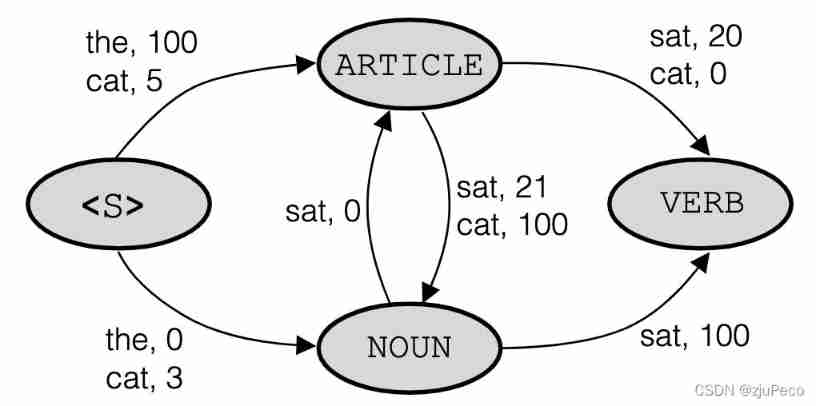

chart 3-3 Logic value reasoning diagram

Normalization is $e^x$ Such exponential normalization , You can start to calculate , Yes and FIG 3-2 The probability value of corresponds to . here [“cat”, “sat”] In this case [“NOUN”, “VERB”] Namely $3+100=103$, and [“ARTICLE”, “NOUN”] It becomes $5+21=26$. I use addition because there are log value .

That's all there is to say , Just to give an intuitive understanding , Want to study carefully , May have a look The Label Bias Problem, Or search for what other big guys say .

4 CRF

4.1 Model overview

With so many mattresses in front ,CRF(conditional random filed) It's easy to understand .MEMM It is the right form $(3-4)$ Modeling , and CRF It is the right form $(4-1)$ Modeling

$$p(y^1,...,y^m|x^1,...,x^m)=p(\bar{y}|\bar{x})\text{\hspace{1em}(4-1)}$$

Attention style $(2-1)$, type $(3-4)$ Sum formula $(4-1)$ The difference between .CRF There is no local normalization , Only global normalization , To put it bluntly, it is a sequence log-linear Model .

$$p(\bar{y}|\bar{x};\bar{w})=\frac{exp(\bar{w}\cdot \bar{\Phi }(\bar{x},\bar{y}))}{{\sum }_{{\bar{y}}^{\prime }\in Y^m}exp(\bar{w}\cdot \bar{\Phi }(\bar{x},{\bar{y}}^{\prime }))}\text{\hspace{1em}(4-2)}$$

among ,$Y^m$ To express with $Y$ The element composition length in is $m$ All possible sets of sequences of .

There are also $\bar{\varphi }$ Turned into $\bar{\Phi }$,$\bar{\Phi }$ For the definition of

$$\bar{\Phi }(\bar{x},\bar{y})=\sum _{j=1}^m\bar{\varphi }(\bar{x},j,y^{j-1},y^j)\text{\hspace{1em}(4-3)}$$

there $\bar{\varphi }(\bar{x},j,y_{j-1},y^j)$ and MEMM The one in is exactly the same , Are artificially defined characteristic functions . It just adds up the whole sequence .

CRF The probability graph model of is shown in the following figure 4-1 Shown , It's like a graph 3-1 Is the difference between the ,$y^j$ Becomes an undirected graph . Or that sentence , It's OK not to look at this picture .

chart 4-1 CRF Probability map

4.2 model training

CRF Model training and log-linear The method of the model is basically the same . In short , We have $n$ Training samples $\{({\bar{x}}_i,{\bar{y}}_i){\}}_{i=1}^n$, Every ${\bar{x}}_i$ They're all sequences $x_i^1,...,x_i^m$, Every ${\bar{y}}_i$ They are all sequences $y_i^1,...,y_i^m$.

Its objective function is

$${\bar{w}}^{\ast }=arg\underset{\bar{w}}{\max }\sum _{i=1}^{n}log(p({\bar{y}}_i|{\bar{x}}_i;\bar{w}))-\frac{\lambda }{2}||\bar{w}|{|}^2\text{\hspace{1em}(4-4)}$$

The next task is the gradient descent .

4.3 Model decoding

CRF Conduct decoding The goal is

$$\begin{array}{rl}arg\underset{\bar{y}\in Y^m}{\max }p(\bar{y}|\bar{x};\bar{w})& =arg\underset{\bar{y}\in Y^m}{\max }\frac{exp(\bar{w}\cdot \bar{\Phi }(\bar{x},\bar{y}))}{{\sum }_{y^{\prime }\in Y}exp(\bar{w}\cdot \bar{\Phi }(\bar{x},{\bar{y}}^{\prime }))}\\ & =arg\underset{\bar{y}\in Y^m}{\max }exp(\bar{w}\cdot \bar{\Phi }(\bar{x},\bar{y}))\\ & =arg\underset{\bar{y}\in Y^m}{\max }\bar{w}\cdot \bar{\Phi }(\bar{x},\bar{y})\\ & =arg\underset{\bar{y}\in Y^m}{\max }\sum _{j=1}^m\bar{w}\cdot \bar{\varphi }(\bar{x},j,y^{j-1},y^j)\end{array}\text{\hspace{1em}(4-5)}$$

$\bar{\varphi }(\bar{x},j,y^{j-1},y^j)$ Part of it is with $y^{j-1}$ Relevant , It's called the transfer feature ; The other part is with $y^{j-1}$ Irrelevant , It's called state characteristics . It's all mixed up here , You don't have to care .

The decoding method is dynamic programming , Also define a $\pi [j,s]$.

The initial probability is

$$\pi [1,y]=\bar{w}\cdot \bar{\varphi }(\bar{x},1,y^0,y)\text{\hspace{1em}(4-6)}$$

The iterative formula of probability is

$$\pi [j,y]=\underset{y^{\prime }\in Y}{\max }(\pi [j-1,y^{\prime }]+\bar{w}\cdot \bar{\varphi }(\bar{x},j,y^{\prime },y))\text{\hspace{1em}(4-6)}$$

Find all the $\pi [j,y]$ after , You can get the path with the greatest probability

$$\underset{y^1,...,y^m}{\max }\sum _{j=1}^m\bar{w}\cdot \varphi (\bar{x},j,y^{j-1},y^j)=\underset{y}{\max }\pi [m,s]\text{\hspace{1em}(4-7)}$$

4.4 Summary

CRF It's solved HMM The irrationality of observation independence , Also solved MEMM in label bias The problem of , And the characteristic function can be added manually to interfere with the output of the model , There are some impossible situations , You can manually set the transition probability to be very small .

Usually the CRF Add to Bi-LSTM after , Make the output of the sequence model more controllable . If there is enough data , If it is balanced ,CRF It can also be omitted .

Reference material

[1] Log-Linear Models, MEMMs, and CRFs
[2] https://anxiang1836.github.io/2019/11/05/NLP_From_HMM_to_CRF/
[3] https://pytorch.org/tutorials/beginner/nlp/advanced_tutorial.html
[4] https://www.bilibili.com/video/BV19t411R7QU?p=4&share_source=copy_web
[5] The Label Bias Problem