[Bayesian classification 4] Bayesian network

1. Knowledge review of semi naive Bayesian classifier

   Semi naive Bayesian classifier The principle of is to properly consider the dependency information between some attributes . The most commonly used strategy to consider is dependent estimation , There is a super - dependent estimation （SPODE）, Average independent dependence estimation （AODE）, Tree augmentation naive Bayes （TAN）.
  
   Dependent estimation of superhusband It is to directly make all attributes depend on the same attribute , This property, which is jointly dependent on other properties, is called “ Superhusband ”, Super husband choice is not always it , Cross validation can be used , We choose the model with the best training effect .
  
   Average independent dependence estimation Is to treat each attribute as a SPODE Model , but $P(c)$ Change into $P(c,x_i)$, But this model requires that the training set be large enough , Define a threshold $m^{\prime }$, requirement $|D_{x_i}|\ge m^{\prime }$.
  
   Tree augmentation naive Bayes , Based on the maximum weighted spanning tree algorithm , Calculate the conditional mutual information between two attributes ,$I(x_i,x_j|y)$ The bigger it is , It means the stronger the dependence .

2. Bayesian network learning notes

2.1 introduction

   Bayesian network is also called “ Faith net ”, It uses directed acyclic graph to describe the dependency between attributes , The conditional probability table is used to describe the joint probability distribution of attributes , It's a probability graph model , Help people apply probability and statistics to complex fields , Tools for uncertainty reasoning and numerical analysis .

   Bayesian network is a directed acyclic graph that describes the dependence between variables from the perspective of conditional probability （DAG）. Reveal the dependencies between variables , Also known as causality （ Is the characteristic of Bayesian network ）, It simulates the uncertainty of causality in human reasoning .

2.2 Knowledge cards

	1.  Bayesian network ：Bayesian Network, abbreviation BN
	2.  Faith net ：belief network
	3.  Conditional probability table ：Conditional Probability Table, abbreviation CPT
	4.  Causal relationship 
	5.  Directed acyclic graph ：Directed Acyclic Graph, abbreviation DAG

2.3 Probability graph model (PGM)

2.3.1 introduction

   Probability graph model （Probabilistic Graphical Model）, Combining probability theory and graph theory , It refers to a probability model that describes the conditional independence between multivariate random variables with a graph structure （ Pay attention to conditional independence ）, So it brings great convenience to study the probability model of high-dimensional space . It can be divided into Bayesian networks and Markov networks .
  
   We hope to be able to mine the knowledge hidden in the data , The probability graph constructs such a graph . The probability diagram directly shows the relationship of conditional independence between random variables .

2.3.2 Why introduce the probability graph ?

   Higher order variables （k Dimensional random variable ）,$Y=[X_1,X_2,...,X_k]$, Suppose each random variable is discrete , Values are $m$ individual . So without any independence , You need to $m^k-1$ Only one parameter can represent its probability distribution , The parameters are exponential .
  
   An effective way to reduce the number of parameters is the independence assumption . First of all, will k The joint probability decomposition of dimensional random variables is k The product of conditional probabilities , that $P(y)={\prod }_{k=1}^{k}P(x_k|x_1,x_2,...,x_{k-1})$. If two variables are independent , Then the condition of conditional probability will be reduced .
  
   example ： It is known that $X_1$ when ,$X_2$ and $X_3$ Independent ,$X_1$ and $X_4$ Independent . be $P(x_2|x_1,x_3)=P(x_2|x_1)$,$P(x_3|x_1,x_2)=P(x_3|x_1)$. Then the joint probability $P(y)=P(x_1)P(x_2|x_1)P(x_3|x_1)P(x_4|x_2,x_3)$.

2.3.3 Three basic problems of probability graph （ Express , Study , infer ）

1. Express problem ： For a probability model , How to describe the dependency relationship between variables through graph structure .
2. Learning problems ： Graph model learning includes graph structure learning and parameter learning .
3. Infer the problem ： When some variables are known , Calculate the conditional probability distribution of other variables .

2.4 Bayesian networks

2.4.1 Expression of Bayesian network

• form

   A Bayesian network $B$ By structure $G$ And parameters $\theta$ Two parts make up , namely $B=<G,\theta >$. Network structure $G$ It's a directed acyclic graph , Each node corresponds to an attribute . If two attributes have direct dependency , Then they are connected by an edge ; Parameters $\theta$ Describe this dependency quantitatively . Suppose the attribute $x_i$ stay $G$ The parent node set in is ${\pi }_i$, be $\theta$ A conditional probability table containing each attribute ${\theta }_{x_i|{\pi }_i}=P_B(x_i|{\pi }_i)$

• Example

   From the network structure in the figure, we can see ,“ Colour and lustre ” Depend directly on “ Good melon “ and " Sweetness ”, and " roots " Is directly dependent on " Sweetness ”,“ Knock sound " Depend directly on " Good melon ”. From the conditional probability table, we can get " roots " Yes " Sweetness " Quantify dependencies , Such as P( roots = Curl up | Sweetness = high )=0.9.

2.4.2 structure

2.4.2.1 Joint probability distribution

   Joint probability distribution of discrete random variables , Bayesian network structure effectively expresses the conditional independence between attributes . Given the parent node set ${\pi }_i$, Bayesian network assumes that each attribute is independent of its non descendant attribute , therefore $B=<D,\theta >$ Attribute $x_1,x_2,...,x_d$ The joint probability distribution of is defined as ：
$$P_B(x_1,x_2,...,x_d)=\prod _{i=1}^d{P}_B(x_i|{\pi }_i)=\prod _{i=1}^d{\theta }_{x_i|{\pi }_i}$$

2.4.2.2 Attribute independent notation

$$x_{3}and{x}_{4}staytoset{x}_{1}Oftakevaluewhensinglestate:x_3\perp x_4|x_1$$

2.4.2.3 Typical dependencies of three variables in Bayesian networks

1. The same parent structure
   Given parent node $x_1$ The value of , be $x_3$ And $x_4$ Conditions are independent .

2. V Type structure
   Give stator nodes $x_4$ The value of ,$x_1$ And $x_2$ There is no need to be independent .
   if $x_4$ The value of is completely unknown , but $x_1$ And $x_2$ But they are independent of each other .

3. Sequential structure
   Given $x$ Value , be $y$ And $z$ Conditions are independent .

2.4.2.4 Moral map

【 introduction 】
  " Moralization " Implication of : Parents of children should build strong relationships , Otherwise it is immoral .

   In order to analyze the conditional independence of variables in a directed graph , You can use “ Directed separation ”, Turn a directed graph into an undirected graph , The undirected graph produced at this time is called moral graph . Based on the moral map can be intuitive 、 Quickly find the conditional independence between variables .

【 step 】

1. Find all of them in a digraph V Type structure , stay V An undirected edge is added between the two parent nodes of a type structure ;
2. Change all directed edges to undirected edges .

【 principle 】
   Suppose there are variables in the moral map $x,y$ And variable sets $z=\{z_i\}$, If the variable $x$ and $y$ Be able to be $z$ Separate , That is to set variables from the moral map $z$ After removing （ Delete nodes and associated edges ）,$x$ and $y$ Belong to two connected branches , It's called a variable $x$ and $y$ By $z$ Directed separation ,$x\perp y|z$ establish .

【 Example 】

Moralization

$x_3\perp x_2|x_1$

2.4.3 Study

2.4.3.1 Mission

   If the network structure is known , That is, the dependency between attributes is known , The learning process of Bayesian network is relatively simple , Just by comparing the training samples " Count ", Estimate the conditional probability table of each node .

   But in real applications, we often do not know the network structure . therefore , The primary task of Bayesian network learning is to find out the most important structure according to the training data set " Appropriate " Bayesian network .

2.4.3.2 Score search

  " Score search " It is a common method to solve this problem . say concretely , Let's first define a scoring function (score function) , To evaluate the fit between Bayesian network and training data , Then based on this scoring function to find the best Bayesian network .

2.4.3.3 Scoring function

• Rule one ： Minimum description length criterion

   Minimum description length criterion （Minimal Description Length, abbreviation MDL Rules ）, The goal of learning is to find a model that can describe the training data with the shortest coding length , At this time, the encoding length includes the byte length required to describe the model itself and the byte length required to describe the data using the model （ The length of the code = The byte length required to describe the model itself + Use this model to describe the byte length required for data ）.

• Application of rule one , Bayesian networks

   Given training set $D=\{x_1,x_2,...,x_m\}$, Bayesian networks $B=<G,\theta >$ stay $D$ The scoring function on can be written as ：
$$s(B|D)=f(\theta )|B|-LL(B|D)$$
【 among 】,

• |B| Is the number of parameters of Bayesian network ;
• $f(\theta )$ Is to describe each parameter $\theta$ Number of bytes required ;
• LL(B|D) It's a Bayesian network $B$ The log likelihood of ,$LL(B|D)={\sum }_{j=1}^{m}log{P}_B(x_j)$.

【 obviously 】,

• $f(\theta )|B|$: Computationally coded Bayesian networks $B$ Number of bytes required ;
• $LL(B|D)$: Calculation $B$ Corresponding probability distribution $P_B$ How many bytes are required to describe D.

【 therefore 】,

• The learning task is transformed into an optimization task .
• Look for a Bayesian network $B$ Make the scoring function $s(B|D)$ Minimum .

【$f(\theta )$】,

• $f(\theta )=1$, That is, each parameter uses 1 Byte description , obtain AIC Scoring function .
• $f(\theta )=\frac{1}{2}logm$, That is, each parameter uses $\frac{1}{2}logm$ Byte description , obtain BIC Scoring function .
• $f(\theta )=0$, Then the scoring function degenerates to negative log likelihood , Corresponding , The learning task degenerates into maximum likelihood estimation .

2.4.3.4 G Fix , For parameters $\theta$ Maximum likelihood estimation of

• Dual transformation

  $s(B|D)=f(\theta )|B|-LL(B|D)$, It's not hard to find out , If Bayesian network $B=<G,\theta >$ Network structure $G$ Fix , Then the scoring function $s(B|D)$ The first term of is a constant , here , To minimize the $s(B|D)$ Equivalent to a parameter $\theta$ Maximum likelihood estimation of .$argmaxLL(B|D)$, because $LL(B|D)={\sum }_{j=1}^{m}log{P}_B(x_j)$,$P_B(x_1,x_2,...,x_d)={\prod }_{i=1}^d{P}_B(x_i|{\pi }_i)={\prod }_{i=1}^d{\theta }_{x_i|{\pi }_i}$

• Parameter calculation formula

   This parameter ${\theta }_{x_i|{\pi }_i}$ Can be directly in training data D Through empirical estimation , namely
$${\theta }_{x_i|{\pi }_i}={\hat{P}}_D(x_i|{\pi }_i)$$

• NP Difficult problem

   therefore , To minimize the scoring function $s(BID)$, Just search the network structure , The optimal parameters of the candidate structure can be calculated directly on the training set . Unfortunately , Searching for the optimal Bayesian network structure from all possible network structure spaces is a NP Difficult problem , Difficult to solve quickly .

• solve

1. The first is the greedy method , For example, starting from a certain network structure , Adjust one edge at a time ( increase 、 Delete or adjust direction ), Until the value of the scoring function no longer decreases .

2. The second is to reduce the search space by imposing constraints on the network structure , For example, the network structure is limited to a tree structure .

2.4.4 infer

2.4.4.1 introduction

   After training, Bayesian network can be used to answer " Inquire about " (query), That is to infer the value of other attribute variables through the observed values of some attribute variables . For example, in the watermelon problem , If we observe that watermelon is green 、 Knock the candle 、 Root curl , Want to know if it is mature 、 How sweet . In this way, the process of inferring the variables to be queried through known variable observations is called " infer " (inference) , The observed values of known variables are called " evidence " (evidence).

   The most ideal is to calculate the posterior probability accurately according to the joint probability distribution defined by Bayesian network , Unfortunately , In this way " To infer exactly " Has been proved to be NP Difficult . In other words , When there are many network nodes 、 When connections are dense , It is difficult to make accurate inferences , At this time, you need to use " Approximate inference ", By reducing accuracy requirements , Obtain an approximate solution in a finite time .

   In practical applications , Gibbs sampling is often used for approximate inference of Bayesian networks （Gibbs sampling）, This is a random sampling method .

2.4.4.2 Gibbs sampling

【 Knowledge cards 】

	1.  Gibbs sampling ：Gibbs sampling
	2.  Gibbs sampling is a random sampling method .
	3.  Gibbs sampling , Used when direct sampling is difficult , Approximate sampling sequence from a multivariable probability distribution .
	4.  The sequence can be used to approximate the joint distribution .
	5. Gibbs Sampling is an iterative algorithm .
	6. Gibbs The core of sampling is Bayesian theory , Around prior knowledge and observational data , The posterior distribution can be inferred from the observed values .
	7.  Gibbs sampling is a kind of Markov chain Monte Carlo （MCMC） Algorithm , It can be seen as MetropolisHastings A special case of the algorithm .
	8.  Gibbs sampling , Each step depends only on the state of the previous step ,, This is a " Markov chain ".
	9. " Markov chain " In steps T  Towards infinity , Must converge （ It must be a stationary distribution ）.
	10.  Gibbs sampling is a special case of Markov chain .
	11.  Markov chains usually take a long time to reach a stable distribution , So the convergence speed of Gibbs sampling algorithm is slow .

【 principle 】

   The basic principle of Gibbs sampling algorithm is through random sampling , Constantly update the model and its position in each input sequence , Optimize the objective function , When certain iteration termination conditions are satisfied or the maximum number of iterations is reached, the final desired motif is obtained .

【 Variable 】

• Make $Q=\{Q_1,Q_2,...,Q_n\}$ Represents the variable to be queried
• $E=\{E_1,E_2,...,E_k\}$ Is the evidence variable
• Its value is $e=\{e_1,e_2,...,e_k\}$
• The goal is to calculate a posteriori probabilities $P(Q=q|E=e)$
• among $q=\{q_1,q_2,...,q_n\}$ Is a set of values of variables to be queried

【 Example 】

• $Q=\{goodmelon,sweetdegree\}$
• $E=\{colorZe,knockThe\; sound,rootTit\}$
• $e=\{greengreen,turbidring,Curl\; upshrink\}$
• $P(Q=q|E=e)$
• $q=\{yes,high\}$
• 【 Find out the probability that this is a good melon with high sweetness ？】

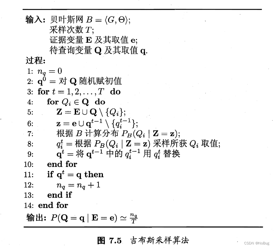
【 The process 】

1. The Gibbs sampling algorithm first randomly generates one with evidence $E=e$ Consistent samples $q^0$ As a starting point ;
2. Then, each step starts from the current sample to generate the next sample .
3. The algorithm first assumes $q^t=q^{t-1}$;
4. Then the non evidence variables are sampled one by one to change their values ;
5. How to change ？ According to Bayesian network $B$ And other variables ( namely $Z=z$) Obtained by calculation ;
6. after $T$ The number of samples obtained from $q$ Consistent samples share $n_q$ individual , be
   $$P(Q=q|E=e)\simeq \frac{n_q}{T}$$
7. T When a large , By Markov chain properties , Gibbs sampling is equivalent to according to $P(Q|E=e)$ sampling , Thus, the probability converges to P(Q=q|E=e)

【 Algorithm 】

3. Bayesian network comb

3.1 Bayesian network understanding

	1.  Bayesian network is a directed acyclic graph that describes the dependence between variables from the perspective of conditional probability （DAG）.
	2.  use G=(V,E)  To represent a Bayesian network , among V  Said variable ,E  Represents the conditional probability between variables , Also called weight .
	3.  Bayesian networks reveal the dependencies between variables , Missing values can be predicted .
	4.  Bayesian network ：Bayesian Network, abbreviation BN
	5.  Probability graph model （ Two categories: ）= Bayesian network + Markov networks 
	6.  characteristic ： Causality between variables 

3.2 Data collection

• Briefly describe the difference between Bayesian network and other probability graph models

   Bayesian network is just a kind of probability graph model , One of the characteristics of it and other probability graph models is , It describes the causal relationship between variables . If time concept is added to the model , Then there can be Markov chains and Gaussian processes . From space , If the random variable is continuous , Then there is a model like Gaussian Bayesian network . Hybrid model plus time series , Then there is hidden Markov model 、 Kalman filtering 、 Particle filter and other models .

• Markov chain

Markov chain

3.3 Bayesian network review

	1.  Bayesian networks , Directed acyclic graph 
	2.  node （ How to solve parameter independence ）, edge （ rely on , How to construct , Three basic dependencies ）, A weight （ Calculation of parameters ）
	3.  How to construct B  Structure 
	4.  Inquire about , Gibbs sampling --> Markov chain