当前位置:网站首页>Machine learning 6-decision tree
Machine learning 6-decision tree
2022-06-28 23:19:00 【Just a】
List of articles
One . Decision tree Overview
1.1 What is a decision tree
Decision tree input : Test set
Decision tree output : Classification rules ( Decision tree )
1.2 Overview of decision tree algorithm

Several common examples of decision trees
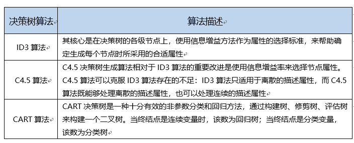
- ID3 Decision tree
- C4.5 Decision tree
- CART classification ( Return to ) Trees

Maximum gain of variable information , Is the most important variable , Put it on the top
There are many values for variables , But it is limited in the training set , So it can be marked
| Age | Separation point | Whether the information gain is maximum |
|---|---|---|
| 12 | ||
| 18 | 15 | |
| 19 | 18.5 | |
| 22 | 20.5 | yes |
| 29 | 25.5 | |
| 40 | 34.5 | |
| If 20.5 It's about , Maximum information gain , Then this is the best separation point |
Two . Construction of a decision tree
2.1 Construction of a decision tree : Divide and rule (divide and conquer)
Decision tree is a typical model with local and global similarity , That is, in any path , Any internal node forms a root node “ Sub decision tree ”. For such a model , Efficient 、 The feasible construction method is divide and conquer . Steps are as follows :
Input : Data sets 𝐷 = ( 𝑥 1 , 𝑦 1 ) , ( 𝑥 2 , 𝑦 2 ) , . . , ( 𝑥 𝑚 , 𝑦 𝑚 ) 𝐷={(𝑥_1,𝑦_1 ),(𝑥_2,𝑦_2 ),..,(𝑥_𝑚,𝑦_𝑚)} D=(x1,y1),(x2,y2),..,(xm,ym) And its characteristic space 𝐴 = 𝑎 1 , 𝑎 2 , … , 𝑎 𝑑 𝐴={𝑎_1,𝑎_2,…,𝑎_𝑑 } A=a1,a2,…,ad
function TreeGenerate(D,A)
- Generate the nodes Node
- If the dataset D All belong to a certain category C, Will 1 The nodes in the Node Divided into attributes C, return
- If A For an empty set , perhaps D stay A The values on are exactly the same , be 1 The nodes in the Node Mark as leaf node , The category is D Most of the categories in , return
- Select the optimal splitting node a,
For each value 𝑎 𝑉 𝑎^𝑉 aV in a:
From the node Node Generate a branch , Make the data set 𝐷_𝑉 yes D stay a The value in is 𝑎 𝑉 𝑎^𝑉 aV Subset
if 𝐷_𝑉 It's an empty set , Then the branch is used as a leaf node , The category is D Most of the categories in , return ;else Generate branch TreeGenerate(𝐷_𝑉, A{a})
End for
This is a typical recursive process , The return condition is :
- The current node contains samples of the same category
- The current property is empty
- All attribute values are the same
- The sample set contained in the current node is empty
The output of the leaf node :
The category with the largest proportion of leaf node output , That is, the category with the highest output probability . If it is transformed to output the corresponding probability of each category , It can be used to calculate the output probability in random forest .
Two questions : How to select the optimal attribute ? How to split nodes ?
The choice of optimal attributes
- Information gain and information gain rate
- gini index
Split node - discrete , There are few types of values
- discrete , There are many types of values
- Continuous type
2.2 Information gain (Information Gain)
The information entropy that measures the purity of categories :
Suppose the sample D pass the civil examinations k The proportion of class samples is 𝑝 𝐾 𝑝_𝐾 pK, be D The entropy of information is defined as
𝐸 𝑛 𝑡 𝑟 𝑜 𝑝 𝑦 ( 𝐷 ) = − ∑ 𝑘 𝑝 𝑘 l o g 2 𝑝 𝑘 𝐸𝑛𝑡𝑟𝑜𝑝𝑦(𝐷)=−∑_𝑘𝑝_𝑘 log_2𝑝_𝑘 Entropy(D)=−k∑pklog2pk
Entropy The smaller it is , The higher the purity
Information entropy :entropy It represents the uncertainty of information In other words, the degree of chaos of the data , Take loans for example ,2 Person overdue ,2 People are the most chaotic when they are not overdue , The uncertainty is the highest , Information entropy is the maximum . The purity is the lowest .
Information gain :
if D By attribute a Divide into 𝐷 = ⋃ 𝑣 𝐷 𝑣 , 𝐷 𝑣 ∩ 𝐷 𝑤 = ∅ 𝐷=⋃_𝑣𝐷_𝑣 , 𝐷_𝑣∩𝐷_𝑤=∅ D=⋃vDv,Dv∩Dw=∅, Define the information gain as :
𝐺 𝑎 𝑖 𝑛 ( 𝐷 , 𝑎 ) = 𝐸 𝑛 𝑡 𝑟 𝑜 𝑝 𝑦 ( 𝐷 ) − ∑ 𝑣 ∣ 𝐷 𝑣 ∣ ∣ 𝐷 ∣ 𝐸 𝑛 𝑡 𝑟 𝑜 𝑝 𝑦 ( 𝐷 𝑣 ) 𝐺𝑎𝑖𝑛(𝐷,𝑎)=𝐸𝑛𝑡𝑟𝑜𝑝𝑦(𝐷)−∑_𝑣\frac{|𝐷_𝑣 |}{|𝐷|} 𝐸𝑛𝑡 𝑟𝑜𝑝𝑦(𝐷_𝑣) Gain(D,a)=Entropy(D)−v∑∣D∣∣Dv∣Entropy(Dv)
Now we have a data set D( For example, loan information registration form ) And characteristics A( For example, age ), be A The information gain is D Entropy and characteristics of itself A Given the conditions D The difference of conditional entropy , namely :
g ( D , A ) = H ( D ) − H ( D ∣ A ) g(D,A) = H(D) - H(D|A) g(D,A)=H(D)−H(D∣A)
Data sets D The entropy of is a constant . The larger the information gain , I mean conditional entropy The smaller it is ,A eliminate D The greater the credit for the uncertainty .
Therefore, features with large information gain shall be preferred , They have a stronger ability to classify . This generates a decision tree , be called ID3 Algorithm .
The role and characteristics of information gain :
- Measure the degree of change from disorder to order ( Commonly used in ID3 Decision tree )
- Select the attribute with the maximum information gain to split
- No generalization ability , Have a preference for attributes with more values
To control the influence of the number of attribute values , First define IV:
𝐼 𝑉 ( 𝑎 ) = − ∑ 𝑣 ∣ 𝐷 𝑣 ∣ ∣ 𝐷 ∣ l o g 2 ∣ 𝐷 𝑣 ∣ ∣ 𝐷 ∣ 𝐼𝑉(𝑎)=−∑_𝑣 \frac{|𝐷_𝑣 |}{|𝐷|} log_2 \frac{|𝐷_𝑣 |}{|𝐷|} IV(a)=−v∑∣D∣∣Dv∣log2∣D∣∣Dv∣
2.3 Information gain rate
When a feature has multiple candidate values , Information gain tends to be too large , Cause error . This problem can be corrected by introducing information gain rate .
Information gain rate is information gain and data set D Entropy ratio of :
𝐺 𝑎 𝑖 𝑛 𝑅 𝑎 𝑡 𝑖 𝑜 = 𝐺 𝑎 𝑖 𝑛 ( 𝐷 , 𝑎 ) 𝐼 𝑉 ( 𝑎 ) 𝐺𝑎𝑖𝑛 𝑅𝑎𝑡𝑖𝑜=\frac{𝐺𝑎𝑖𝑛(𝐷,𝑎)}{𝐼𝑉(𝑎)} GainRatio=IV(a)Gain(D,a)
characteristic :
It is easy to tend to attribute with few values
The attribute with the maximum gain rate can be selected for splitting
You can select an attribute set that is greater than the average gain rate , Then select the attribute with the lowest gain rate
2.4 gini index
Another measure of purity
𝐺 𝑖 𝑛 𝑖 ( 𝐷 ) = 1 − ∑ 𝑘 𝑝 𝑘 2 𝐺𝑖𝑛𝑖(𝐷)=1−∑_𝑘𝑝_𝑘^2 Gini(D)=1−k∑pk2
Gini The smaller it is , The higher the purity
attribute a In the data set D The Gini index in is
𝐺 𝑖 𝑛 𝑖 ( 𝐷 , 𝑎 ) = ∑ 𝑣 ∣ 𝐷 𝑣 ∣ ∣ 𝐷 ∣ 𝐺 𝑖 𝑛 𝑖 ( 𝐷 𝑣 ) 𝐺𝑖𝑛𝑖(𝐷,𝑎)=∑_𝑣\frac{|𝐷_𝑣 |}{|𝐷|} 𝐺𝑖𝑛𝑖(𝐷_𝑣) Gini(D,a)=v∑∣D∣∣Dv∣Gini(Dv)
Select the attribute with the minimum Gini index , namely 𝑎 ∗ = 𝑎 𝑟 𝑔 𝑚 𝑖 𝑛 𝐺 𝑖 𝑛 𝑖 ( 𝐷 , 𝑎 ) 𝑎_∗=𝑎𝑟𝑔𝑚𝑖𝑛 𝐺𝑖𝑛𝑖(𝐷,𝑎) a∗=argminGini(D,a)
2.5 Example
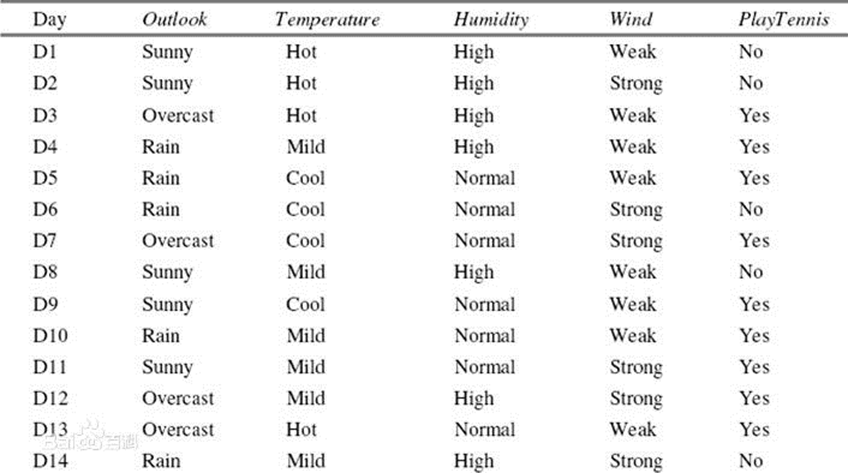
A simple example : With variable outlook,temperature,humidity,wind Come on playtennis To classify .
about outlook, Its information gain rate is calculated as :
(1) The calculation of the total entropy :
P(PlayTennis=Yes) = 9/14, P(PlayTennis=No) = 5/14
Entropy = -9/14*log2(9/14) – 5/14*log2(5/14) =0.9403
(2) Put the dataset D according to Outlook division , The result is :
D1: Outlook=Sunny Yes 5 Samples , among PlayTennis=Yes Yes 2 Samples ,PlayTennis=No Yes 3 Samples
Entropy1 = -2/5*log2(2/5)-3/5*log2(3/5) =0.9710
D2: Outlook=Overcast Yes 4 Samples , among PlayTennis=Yes Yes 4 Samples ,PlayTennis=No Yes 0 Samples
Entropy2 = -0/4*log2(0/4)-4/4*log2(4/4) =0 ( Definition 0*log2(0)=0)
D3: Outlook=Rain Yes 5 Samples , among PlayTennis=Yes Yes 3 Samples ,PlayTennis=No Yes 2 Samples
Entropy3 = -3/5*log2(3/5)-2/5*log2(2/5) = 0.9710
(3) Calculation IV: IV=-5/14*log2(5/14)-4/14*log2(4/14)-5/14*log2(5/14)= 1.5774
(4) Calculated information gain :Gain = 0.9403-5/14* 0.9710-4/14*0-5/14* 0.9710= 0.2467
(5) Calculate the information gain rate :Gain Ratio= 0.2467/ 1.5774= 0.1564
Calculation Outlook Of Gini:
(1) Calculation D1,D2 and D3 Of Gini:
Gini1 = 1-(2/5)2-(3/5)2=0.4800,Gini2 = 1-(4/4)2-(0/4)2=0
Gini3 = 1-(2/5)2-(3/5)2=0.4800
(2) Calculate the total Gini:
Gini(D)=5/140.4800 + 4/140 + 5/15* 2=0.4800= 0.3086
2.6 Processing of continuous variables
Continuous variables are discretized by dichotomy , And then treat it as a discrete variable .
3、 ... and . Prevent fitting : The art of pruning
There's a good chance , All attributes are split , Easy to create over fitting
Avoid overfitting , Need pruning (pruning). Two methods of pruning
- pre-pruning
In the process of decision tree generation , Each node is estimated before partition , If the current node partition can not improve the generalization performance of the decision tree , Then the partition is stopped and the current node is marked as a leaf node - After pruning
First, a completed decision tree is generated from the training set , Then investigate the non leaf nodes from bottom to top , If the subtree corresponding to this node is replaced with leaf nodes, the generalization performance of the decision tree can be improved , Replace the subtree with a leaf node
** Generalization ability :** The adaptability of the algorithm to fresh samples . You can use the set aside method , That is, select a part of the training set that does not participate in the construction of the decision tree , It is used to evaluate the test of a certain node partition or subtree merging .
Four . A combination method to improve the accuracy of classifiers
4.1 Overview of combination methods

Why combination method can improve classification accuracy 
Advantages of combinatorial algorithms 
4.2 Bagging algorithm

There's put back sampling :
Advantages of bagging algorithm :
4.3 promote (boosting) Algorithmic thought

Adaboost Algorithm :

Advantages and disadvantages of the lifting algorithm :
4.4 Random forests
Decision tree reinforcement algorithm : Random forests
4.4.1 The basic concept of random forest
Random forest is a kind of integrated model . It consists of several decision trees , The final judgment result is decided by simple voting based on the result of each decision tree .
4.4.2 Data set extraction
In the process of building a random forest model , The key step is to extract some samples from the original data set to form a new training set , And the sample size remains unchanged . The subsequent construction of each decision tree model is based on the corresponding sampling training set .
“ Random forests ” Medium “ Random ” The two characters are mainly reflected in 2 aspect :
- When extracting data from the overall training set , The sample is taken back .
- After forming a new training set , And then extract some attributes from the attribute set without putting them back to develop the decision tree model
These random operations can enhance the generalization ability of the model , The problem of over fitting is effectively avoided . And other models ( For example, maximal gradient lifting tree ).
stay 1 in , Every time a data set with the same sample size is generated by putting it back , There are about 1/3 The sample of is not selected , Reserved for “ Out of bag data ”
stay 2 in , Assuming the original m Attributes , In the 2 The general choice in this step is log_2𝑚 Attribute for decision tree development .
4.4.3 Fusion of decision tree results
After getting several decision trees , Will fuse the results of the model . In random forests , The method of fusion is usually simple voting . hypothesis K The votes for each decision tree are 𝑡_1, 𝑡_2,…,𝑡_𝐾, 𝑡_𝑖∈{0,1}, The final classification result is 
The output probability of random forest
At the same time, random forest also supports the output of results in the form of probability :
Reference resources :
- http://www.dataguru.cn/article-4063-1.html
- https://zhuanlan.zhihu.com/p/76590801
边栏推荐
- Matlab learning notes (6) upsample function and downsample function of MATLAB
- 【剑指Offer】50. 第一个只出现一次的字符
- [API packet capturing in selenium automation] installation and configuration of browsermobproxy
- 全面掌握const的用法《一》
- That's how he did it!
- Design e-commerce seckill system
- CPU、GPU、TPU、NPU区别
- Tanghongbin, Yaya live CTO: to truly localize, the product should not have the attribute of "origin"
- Prometeus 2.36.0 新特性
- 网上注册股票开户很困难么?在线开户是安全么?
猜你喜欢

See fengzhixia | FENGZikai, the originator of Guoman, for exclusive sale of Digital Collections

Deep virtual memory (VM)

Cs5463 code module analysis (including download link)
Leetcode detailed explanation of stack type

Chapter IV memory management exercise
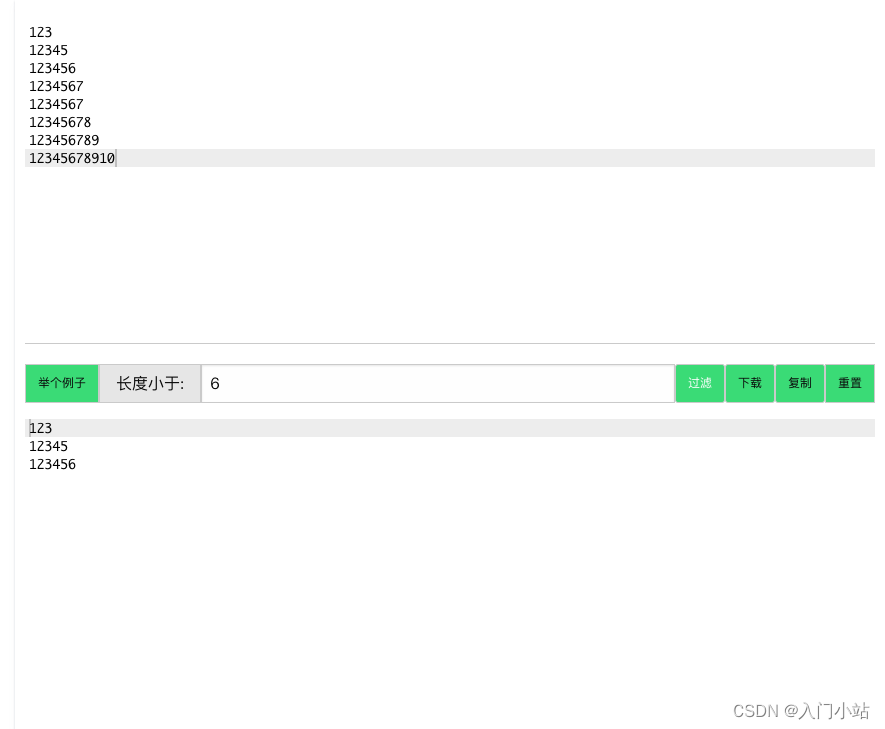
Online text filter less than specified length tool

Wave picking of WMS warehouse management system module

Chapter III processor scheduling exercise

What is the difference between WMS warehouse management system and ERP

ERROR 1067 (42000): Invalid default value for ‘end_time‘ Mysql
随机推荐
在长投学堂开通证券账户是安全可靠的吗?
Design e-commerce seckill system
复杂嵌套的对象池(4)——管理多类实例和多阶段实例的对象池
Count the number of arrays with pointers
【深度学习】(3) Transformer 中的 Encoder 机制,附Pytorch完整代码
全面掌握const的用法《一》
2022年PMP项目管理考试敏捷知识点(4)
论文解读(DCN)《Towards K-means-friendly Spaces: Simultaneous Deep Learning and Clustering》
机器学习4-降维技术
小样本利器2.文本对抗+半监督 FGSM & VAT & FGM代码实现
A password error occurred when docker downloaded the MySQL image to create a database link
[stm32 HAL库] RTC和BKP驱动
WEB API学习笔记1
网上注册股票开户很困难么?在线开户是安全么?
MSCI 2022 market classification assessment
第二章 经典同步练习作业
机器学习6-决策树
Tanghongbin, Yaya live CTO: to truly localize, the product should not have the attribute of "origin"
【深度学习】(2) Transformer 网络解析,代码复现,附Pytorch完整代码
Go language - reflect