Large scale real-time quantile calculation -- a brief history of quantitative sketches

Focus on   Dry goods don't get lost  

Concept and introduction

Preface

In the field of data , There are several classic query scenarios ：

1. Want to count the number of visits to a website within a certain period of time UV Count , Or statistics of the pages visited in a certain period of time A Visited the page again B Of UV Count , Or it can count the pages visited in a certain period of time A But the page was not visited B Of UV Count , Usually we call this kind of query cardinality statistics .

2. Want to observe the data distribution of some indicators , For example, statistics of pages visited within a certain period of time A And page B Respective browsing time 95 quantile 、50 quantile , You need to use quantile statistics .

3. You want to count the most played or the most clicked in a certain period of time 10 A video or article （ Hot list ）, You need to use TopN Statistics .

These kinds of problems are very easy to deal with when the amount of data is small . We can do this by traversing + Sorting solves this problem easily and accurately . But once the data arrives Billion Magnitude , Conventional algorithms can take hours or even days , And even providing sufficient computing resources will not help , Because these kinds of problems are difficult to parallelize .

DataSketches[1] It is a group of algorithms born to solve these typical problems in big data and real-time scenarios , Originally open source by Yahoo . These algorithms sacrifice the accuracy of query results , It can be parallelized in a very small space 、 Quickly solve the above problems .

Sketch The core idea of structure

Sketch Structure is 「 Data sketches 」 structure , It is a data structure designed to calculate the probability index of massive streaming data . It usually occupies a fixed size of memory , Does not increase with the amount of data . This structure is achieved by skillfully storing or discarding some data , Store the information of data flow abstractly , Sum up Sketch structure , Finally, according to Sketch Structure restore the distribution of the initial data , Realize cardinality Statistics 、 Quantile calculation and other operations .

Sketch、Summary Can be understood as data sketches , The names used in different papers are not quite the same , But symbols are usually capitalized S.

Sketch Generally, it has the following characteristics ：

1. Single traversal

You can put Sketch Understood as a state memory , It always carries all the historical information of the data stream so far , therefore Sketch Usually single-pass Of , You only need to traverse the data once to get the required statistical information .

2. Small footprint

Traditional statistical methods need to maintain a huge data list , And as the data input becomes larger and larger .Sketch You can consume a large amount of data in a small constant space , Usually in KB Magnitude . This makes Sketch It has great advantages in the statistics of massive data .

For a database containing hundreds of millions of data 、 A dataset that contains a combination of multiple dimensions , It can be transformed into one on each dimension combination KB The size of Sketch structure , So as to speed up the query .

3. Consolidatability

Consolidatability makes Sketch Be free to Distributed parallel processing Large amount of data , Therefore, it has a fast 、 The advantage of efficiency . Base statistics (Distinct Value, DV) For example , The problem to be solved is to find the number of different elements from the data stream with repeated elements ,Sketch Local statistical results can be easily merged into global statistical results , Direct counting does not do this , namely ：

DV(uid | city= Beijing or Shanghai ) ≠ DV(uid | city= Beijing ) + DV(uid | city= Shanghai )

Sketch(uid | city= Beijing or Shanghai ) = Sketch(uid | city= Beijing ) + Sketch(uid | city= Shanghai )

PS: The plus sign in the second expression represents Sketch Merge operation of .

In Distributed Computing , Two different machines Sketch The local statistical results of can be directly passed through a Query Methods are merged into one Sketch structure , Perform the final quantile query .

4. Error controllable approximation

Sketch In order to save space, some information will be lost , Therefore, the statistical results cannot be completely accurate . But in reality , Many analyses and decisions do not require data to be absolutely accurate , Sometimes you know that certain statistics are 1% Is often as valid as an accurate answer .Sketch A trade-off can be made between computational complexity and error , It can meet most of the statistical needs in the big data scenario .

One Sketch The use process of the algorithm is usually as follows ：

The original data is transformed into a Sketch structure , When you want to query , from Sketch Generate a Estimator Return query results

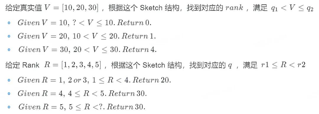
Quantile The definition of

Quantile / quantile （Quantile）： Consider the error approximation , That is, the given error ε And quantile φ, You only need to give a sorting interval [(φ - ε)*N, (φ + ε)*N] Any element in the (N Is the number of elements ）.

for instance , If a given input The sequence is as follows , stay ε= 0.1 Under the circumstances , seek PCT50（ namely φ = 0.5）. return 24、39、51 Can meet the conditions . But if ε= 0.01, Only return to 39 Is the right result .

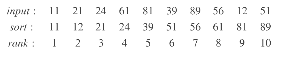
φ= 0.5 and ε = 0.1

Rank = [4, 5, 6] → V = [24, 39, 51]

That's why we use DoublesSketch UDF perhaps Spark The quantile calculation result may be inaccurate when using the quantile approximation algorithm . Besides , Different quantile location methods will also lead to subtle differences in data , It will be mentioned later .

In the figure , There are only two pieces of data under the current dimension , For these two data, calculate 50 Quantile results will be different . When solving the quantile problem with small cardinality , There will be large errors in the data .

Quantile The error of the

quantile and rank It's actually two functions ：

We expect a perfect pair of functions , bring q = quantile(rank(q)) perhaps r = rank(quantile(r)), But in reality , We often get only two functions with errors r' = rank(q) and q' = quantile(r)

The quantile problem is actually quantile(r) problem , I.e. given r, According to the estimation quantile Function to find q'.

The error of the function is caused by many ways ：

1. Massive data will inevitably lead to the need for conditional integration and filtering of data , This leads to errors . But reasonable integration 、 The filtering mechanism can control the error within a certain range . So , countless researcher Contributed a variety of idea, This is also the main content of the second half of the document .

2. Repeated values can also cause errors . But actually , If we make correct assumptions about the definition and boundary conditions of quantiles , Then this error has been considered in the algorithm , This article will not explain in detail . Give us a simple example to feel , How different quantile location methods and repeated values bring about errors ：

Example

There are five data inputs to calculate the quantile ：{10, 20, 20, 20, 30}

On the top is the value and position map of the sorted original data , The following can be imagined as a simple store of these data Sketch structure .

There are two rules for locating the quantile when calculating the quantile ,LT (less-than) and LE (less-than or equals). There are differences between the two in the examples , But when it comes to generalization, there is little difference , Are within the acceptable error range , In this example we compare LT and LE Results under Rule , Can be found in duplicate values 20 Upper Rank' and Quantile' It's different , And the value on the boundary Rank' and Quantile' There are also errors .

LT (less-than) & GT(greater-than)

LE (less-than or equals) & GE(greater-than-or-equal)

Want to know LT and LE The differences between rules can be viewed DataSketches The official website is about Quantiles The definition of [2]

industry Quantile Realization

Quantile Sketches Through layer upon layer iteration and continuous evolution , Many varieties have been formed . With Apache DataSketches Implementation summary in [3] For example , quite a lot Sketches Algorithms have already been used in applications such as Spark、Hive、Druid And so on , When we're in SQL Call in percentile Class function , Different frameworks will call their corresponding algorithms . However, different frameworks implement different algorithms , The efficiency of implementation is also high or low , Eventually, the difference in computing speed will be obvious when using .

KLL and GK The algorithm should be the most widely used algorithm at present . here , We select the two most commonly used frameworks in two big data development scenarios Spark and Hive For example , Compare the quantile calculation function percentile_approx With one by Apache DataSketches Algorithm implementation provided , And briefly explain how to Apache DataSketches Provide more efficient algorithms to be introduced into daily development work .

Spark

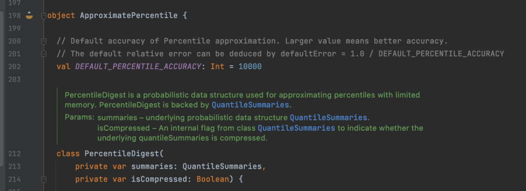
stay Spark There is no need to introduce UDF,Spark Medium ApproximatePercentile[4] Class implements the GK Algorithm , With QuantileSummaries[5] As data Sketch, It will be mentioned later GK Algorithm and simply explain its concept . The calculation efficiency of this function is relatively fast when the amount of data is small .

Hive

Again , stay Hive The original quantile calculation method can be directly used to calculate the quantile in , But the algorithm behind this method does not Spark The algorithm in is efficient .Hive Medium GenericUDAFPercentileApprox[6] The quantile is estimated by calculating the approximate data histogram . Such as Hive Source tip , This function may exist when there is a large amount of data OOM The problem of . Besides ,Hive The algorithm of histogram estimation is mainly based on A Streaming Parallel Decision Tree Algorithm[7]. It is worth mentioning that , The core idea of this algorithm is how to construct the histogram of data in limited memory .

DataSketches

In the face of massive data ,Spark The original quantile calculation function will be weak , It is recommended to introduce DataSketches Provided quantile calculation method . The algorithm is not only better in space occupation , Its computational efficiency is also higher .DataSketches Of DoubleSketch[8] It's based on Mergeable Summaries[9] Mentioned in Low Discrepancy Mergeable Quantiles Sketch algorithmic . This paper mainly discusses what is Mergeability And to the previous famous algorithm Mergeability To prove . At the same time, a combined sampling method is proposed Randomized Mergeable Quantiles Sketch Algorithm .

As a big data development student , For this algorithm, we need to understand the following points ：

1. This algorithm Sketch The structure can be distributed .

2. Because the algorithm introduces random , The result may be different each time （ But you can fix it by specifying random seeds ）.

3. The algorithm is implemented by compression 、 Bitmap and other operations further save time and space .

4. If you can use this algorithm, use this algorithm , Very fast ！

It is also easy to implement the algorithm into daily development ,Datasketches A variety of UDF、UDAF, It can basically meet common business needs . You need to be in pom Add... To the document org.apache.datasketches rely on , Then, according to the business needs , Yes datasketches Provided UDF、UDAF Packaging again . Pack it up jar Package and register UDF after , You can go to SQL Used in .

Quantile Sketches The evolution of the algorithm

Problem definition

Quantile Sketches The algorithm can be traced back to the last century 90 years , When the concept of streaming data and distributed computing has just been widely recognized in the academic community , The question was thrown out . How to deal with massive data , Even infinite data , Use limited space , Find one of them rank Corresponding value , Or find a number corresponding to rank.

Quantile Sketches The development of algorithms is based on the introduction of important algorithms , Several important stages have been formed . actually , The initial goal of this field is how to use the minimum memory space , Solve one of the most generalized problems .

What is the most generalized problem ？ Academic circles call this kind of problem All Quantiles Approximation Problem, Its definition is as follows ：

Corresponding to the most generalized problem , The narrow question is called Single Quantile Approximation Problem. Of course, there are many variants of the problem , for example , Given rank Find the corresponding value （ The most common quantile problem ） Or solve with known stream data size rank Or quantile, etc .

After defining the problem , It is also necessary to define the algorithm clearly , A qualified Quantile Estimators It should have the following four characteristics ：

1. Provide adjustable 、 Can be defined as the error interval .

2. Independent of input data .

3. Traverse all data only once .

4. Use as little memory as possible .

Eligible Estimator There is no explicit requirement for consolidatability ,mergeability Just one. nice to have Characteristics of . The problem definition does not consider mergeability The problem of , So some algorithms are not implemented mergeability, As a result, it can not fully adapt to the distributed computing mode in actual production . Even if it fits , More space is often needed , Higher computational complexity .

Where is the end point of space optimization ？

Industry and academia often have the same methodology for exploring the unknown ： First find out where the ceiling with the minimum memory consumption is . By constructing a special counter data stream and proving that in extreme cases , Minimum memory required by any algorithm . How to find the ceiling of this problem is not the focus of this article , Interested readers can read the paper An Ω (1/ε log 1/ε) Space Lower Bound for Finding ε-Approximate Quantiles in a Data Stream[10] Learn more .

Starting from compression - MRL Algorithm [11]

The simplest compression

Data discarding

Think back to the examples mentioned when explaining the basic concepts , We can feel it intuitively ,Sketch One of the characteristics of data structure is the reasonable compression of data . The compressed data can fully restore the original distribution of the data as far as possible . In order to realize this principle , The most intuitive idea is to discard or retain each input data through certain rules , And ensure that the error is controlled within ε within . The problem then becomes how to find the appropriate discard rules .

for instance , According to the data index To determine whether to discard ： For an unsorted data stream , Discard all even digits , And keep the odd digits . But this is obviously a flawed approach , And it's easy to prove ： Just build a data flow , Put all smaller data in even digits , The data left are all large data , The smallest data will also be greater than or equal to the median .

Get inspiration from this example , We can sort the data flow first , Then discard the data according to the above principles , Then this method becomes feasible .

Weight increase

Another obvious logic is , Discarded data cannot be simply discarded , Its information must in some way be stored in data that is not discarded . Continue with the above example , Data at even positions is discarded , You can increase the weight of the previous odd position data at the same time , Make an odd digit represent an original odd digit + Even digit number . such , The data volume information is saved , The greater the weight , Which means that the more data in this area .

Batch thought

However, stream data does not support real-time sorting , And as the data scale increases , The time and space cost of sorting will increase . A natural idea is , Stream data can be divided into one by one batch, In every one of them batch Internal sorting .

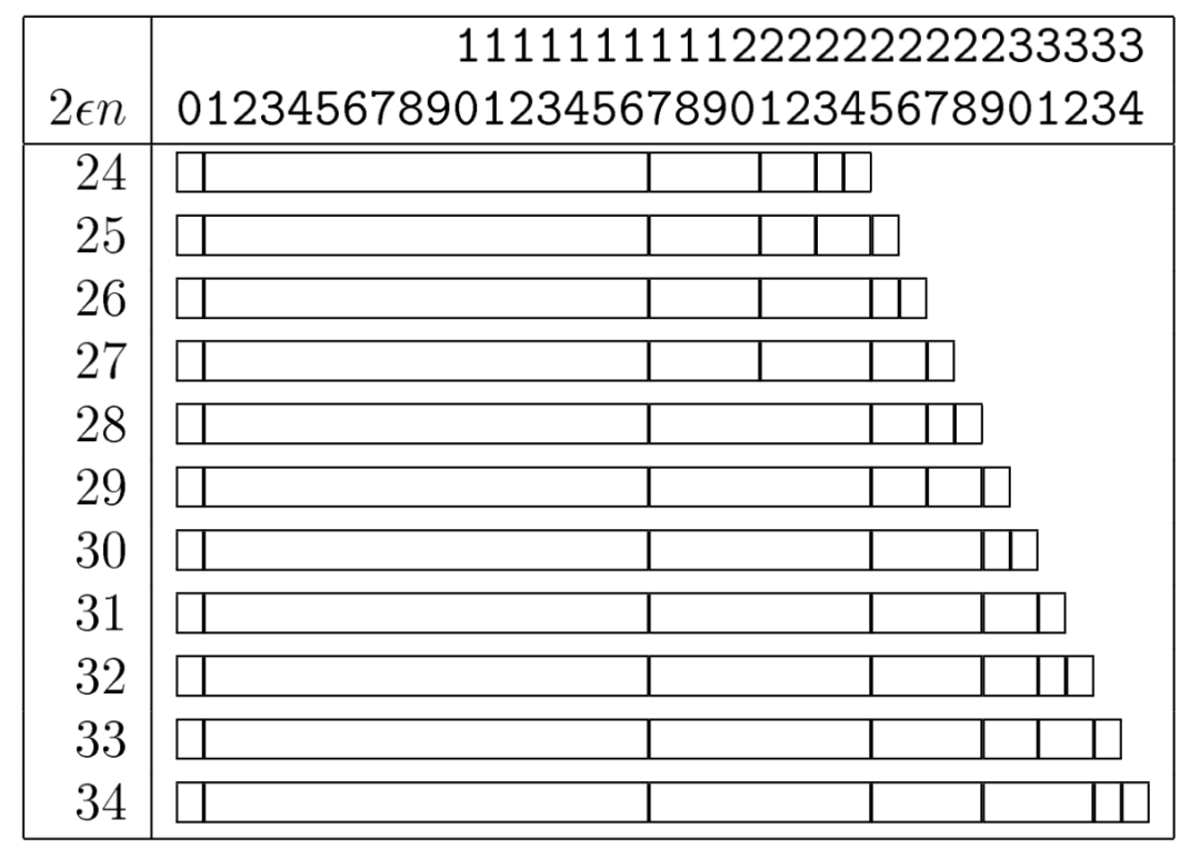
The example in the following figure combines the two strategies of data discarding and weight increasing . among , The first line is that the input data is cut into small pieces batch And after internal sorting . The second line indicates that all even bits of data are discarded , And increase the weight of the previous odd digit data （ The height of the small square has doubled ）. The third line means to discard all odd data , And increase the weight of the last even digit data . Can be observed , In some places Rank Change , If Compactor When the internal data is even Rank No change , If it is an odd number, it will be relatively plus or minus one . Follow this process to build the simplest Sketch structure .

Single batch The idea of data compression has been preliminarily verified , So here comes the question , Single batch How to deduce to multiple batch Even on streaming data ？

Compress and merge

Let's say I have two Sketch structure , What we want to achieve is , When these two Sketch After the structure is merged into one , Still able to provide accurate Rank.

As shown in the figure below , The red dot indicates the data s_i < v, When we put two Sketch After the structure is merged, it is found that ,v In the merged dataset Rank That's two Sketch Count the sum of the number of red dots , Merge data sets Rank Will not change due to split statistics .

therefore , We get two corollaries ：

But if you simply splice the two sets of data together , Obviously, it will face the problem of increasing space cost caused by the increase of data volume . At this point, I will return to the compression mentioned before 、 The idea of merger , This process can be cycled continuously , The combined 、 Compress 、 Re merger 、 Compress again ……

MRL Introduction to the principle of the algorithm

Random Sampling Techniques for Space Efficient Online Computation of Order Statistics of Large Datasets[11]（MRL Algorithm ） Is compressing 、 The combination of ideas to be improved .MRL The algorithm constructs a tree multi-level compression and merging structure ：

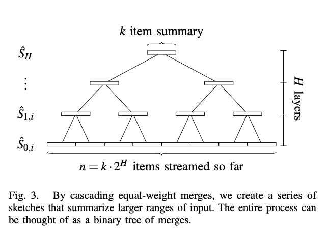
Select a fixed size k As Sketch Size of structure . According to the amount of stream data, the number of layers to be compressed can be deduced H. obviously ,k The larger the compression level, the less , The less information is lost , The more accurate the result is .

The process is simple , Raw stream data output to level0 One of the Sketch In structure , When the data is full, the size is k Of Sketch After structure , If level0 Nothing else Sketch, Then this Sketch Temporarily cache , Wait for another Sketch arrival . If there is another Sketch, Two Sketch After merging and sorting, keep the data of all odd positions , take 2k The size of the data is compressed to k Size and pass it to the next level . Again , If the next level already has one Sketch, Then do a similar merge sort and discard the compression , take Sketch Pass to the next level , Step by step .

k The size of directly affects the accuracy of data , It even determines whether the algorithm can converge , The appropriate value is k = O(ε^{−1} _ log^2(εn)).MRL The algorithm only needs two at each level Sketch Structure stores data . The number of levels determines the total space required , The layer series is based on the total amount of data and a single Sketch The structure size is deduced ：

O(H) = O(log^2(n/k)) = O(log^2(εn)), Total space O(kH) = O(ε^{-1} _ log^2(εn)).

Starting from sampling - Sample Algorithm [12]

If there are 100 million figures , We want to compare one of the numbers x Beg him Rank How much is the ,Reservoir-Based Random Sampling with Replacement from Data Stream[12] Tell us , Through random sampling, we can use the following formula to estimate the overall Rank：

But this is an approximate formula . A rigorous algorithm needs to be clear , How similar is this thing . There happens to be an inequality Hoeffding's inequality And according to Hoeffding's inequality This theorem is derived

As the user , Being able to understand proof is the best , Therefore, the guide to this article VI part [13]. But if you don't understand the proof , So the following passage will tell you what this certificate did , What's the significance （ Personal understanding , There may be inaccuracies , Welcome to correct ）.

Essentially ,Hoeffding's inequality given The upper limit of the probability that the sum of random variables deviates from its expected value . This inequality is a Bernoulli A derivation of the process （ About Hoeffding's inequality More detailed directions here [14]）. This random sampling can be used to estimate a number Rank There is also a connection （ Upper limit of error ）. This upper bound happens to limit the estimation error to a certain range , To satisfy the Quantile Sketch Algorithm requirements . Moreover, the sampling process will Rank Results and data volume n Independent . The error of the result depends only on m. and m Is a number we can set , let me put it another way ,m Is a memory size that we can set , This memory size determines the estimated after sampling Rank Upper limit of error .

Can be observed , The memory required here is greater than MRL Algorithm . But its biggest significance is that it removes the relationship between the size of the data and the size of the data n The relationship between . Just to be clear , This kind of sampling needs to know the size of data in advance n, If you don't know the amount of data n, Sampling is still useful , However, it is necessary to reduce the sampling probability as the amount of data increases . For details, see [13]

Starting from the structure - GK Algorithm [15]

Summary The structure design

GK Algorithm Space-Efficient Online Computation of Quantile Summaries[15] The inspiration for this idea comes from the following ： Suppose that the first number of stream data we receive is the median , Then we only need to count the quantity greater than this number and the quantity less than this number with the data input , Finally, it is easy to verify whether this number is the median . Can we talk about k All the input data keep the same structure , Record the number of data larger than this structure and the number of data smaller than this structure , Then you can find the corresponding number Rank How much is it .

There is a structure , every last tuple Store real values 、 Minimum Rank、 Maximum Rank, every last tuple It's called Summary：

For arbitrary data , As long as the following formula is satisfied , Then the overall error of the algorithm is convergent .

But this structure is flawed . When processing stream data , If the new data needs to be inserted into the middle , So every time you need to update all the following Summary. The complexity of this update is too high .GK The algorithm proposes a more friendly method for inserting data Summary structure ：

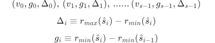
Convert absolute position into relative position for representation .

• g Indicates two adjacent Summary Relative position difference of , according to g And a starting point, we can deduce the starting point and Summary What is the distance between .

• Δ Express this Summary Covered Rank What's the scope of .

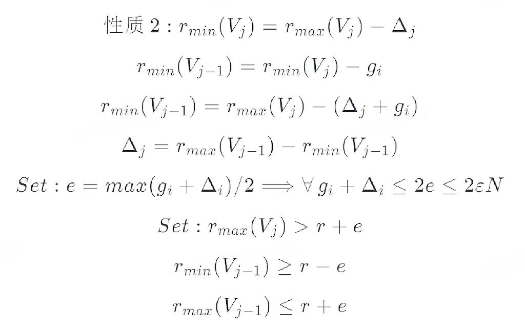
According to the above definition, the following three properties can be deduced , The detailed inference will not be repeated here , If you are interested, please read this article [16][17]

combination Summary Structure

After a bombardment of data formulas , It seems that I can't touch it again GK What is the algorithm doing . If you want to know GK Details of the algorithm , Guide the original paper [15]. But if you just want to understand the idea of the algorithm , So it doesn't matter , The following passage tells you what you are doing all this time .

Just like the addition, deletion, modification and query of the database , Build such a special Summary Structure and push to so many properties , Just to be faster 、 It is more convenient to perform the following operations ：

1. Construct a Summary + A special INSERT() Method -> Makes updating data especially fast .

2. Construct a Summary + A special QUERY() Method -> Make the query satisfy the error constraint .

3. Construct a Summary + A special DELETE() Method + A special COMPRESS() Method -> Keep the space constant and optimal .

INSERT

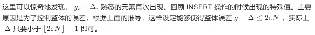
The maximum and minimum cases are well understood . In general , Newly inserted data i Obviously i-1 Any previous data has no effect , But each of the following data Rank Should add one , therefore g = 1. The subtlety is that the change of absolute position is expressed by the accumulation of the change of relative position .Δ = g_i + Δ_i - 1 The reasons will be mentioned later .

QUERY

All Quantiles Approximation Problem One property that must be satisfied is all x All should be satisfied |R'(x) − R(x)| ≤ εn, The vernacular explanation is , When we initiate a query （ Inquire about x Corresponding Rank） The error of the return value should be kept in a linear relationship proportional to the amount of data .

Ingenious query setting can control the overall error within the convergence range .

DELETE and COMPRESS

Facing massive data , It is obviously unreasonable to simply add information without compressing or deleting it . The deletion rules are as follows ：

The delete operation only changes v_i+1 Where Summary Of g_i+1, It doesn't change Δ_i+1. in other words Δ The smaller it is , Under the constraint of error , There are more merging Summary The potential of .

In order to compress data more efficiently GK The algorithm proposes Fullness、Capacity and Bands Three concepts .

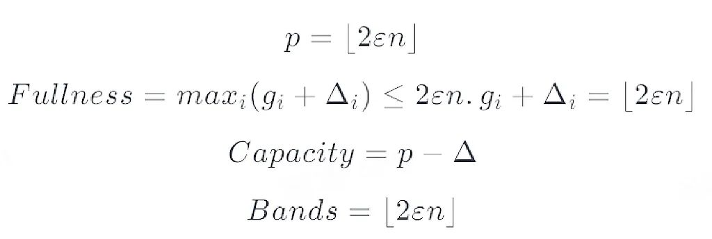
The birth of these three concepts is to assist in COMPRESS Operation of the , In short , Every Summary Corresponding Capacity size , Look from right to left , The scale increases exponentially , The compression is also carried out from right to left . The following figure shows the different sizes Sketch Corresponding to each small Summary Of Capacity Size relationship ,

The following pseudocode shows a compression process . When the compression conditions are met , Yes Summary Structures are merged from right to left , bring Summary Try the least memory method first .

After the compression conditions are met , adjacent Summary after COMPRESS After the operation , Update data to Band Smaller value Summary On . because DELETE The operation does not change Δ Characteristics of , If you keep Band Worth a lot of money Summary structure , Then there is a bigger Capacity, Later, it will be able to accommodate more Summary（ There will be more Summary Compressed together ）.

Besides ,GK The algorithm also introduces a tree model , Traversing a binary tree by right preorder , Realize fast and orderly for child nodes COMPRESS To the parent node , however , No more details here , Interested students can show the way to the original paper [15].

It should be noted that ,GK The algorithm is a mergeable The algorithm of , To be precise , It's a One-way mergeable The algorithm of .

One-way mergeability is a weaker form of mergeability that informally states that the following setting can work: The data is partitioned among several machine, each creates a Summary of its own data, and a single process merges all of the summaries into a single one. let me put it another way ,One-way mergeability merge The algorithm cannot be distributed , Otherwise, the error is not within the controllable range , and Fully mergeable Our algorithm can , Although the description of this point in the paper is not particularly clear , But the detailed proof points the way [18][19][20].

GK What's good about it ？

Said so much GK Principle of algorithm , What's good about this algorithm ？

• GK The algorithm stores data information in a unique way , It realizes the efficient query of massive data , Efficient insertion .

• GK In the original tree model, different levels and sizes are introduced into the algorithm Summary structure , More efficient use of space .

The beginning of integration - ACHPWY Algorithm [9]

The ancient Chinese saying is often said , Extract its essence , Discard the dregs . The latter algorithm actually implements this idea .ACHPWY Algorithm Mergeable Summaries[9] Of Low Discrepancy Mergeable Quantiles Sketch It's based on MRL Derivative algorithm of the algorithm . stay MRL Random sampling is added to the algorithm , Make the final Quantile Estimator Is an unbiased Estimator.ACHPWY The overall architecture and MRL Algorithm is the same , All adopt the same size as k Of Sketch structure , Form a multi-level tree model . The only difference is , It's going on Sketch When merging , Introducing random variables F To decide whether to take odd position data or even position data .

Original MRL The algorithm only takes odd digits in any combination , Random introduction brings unbiased Estimator, And bring less space to use . As explained above , If it is necessary to discuss the upper limit of the probability of the deviation between the sum of random variables and their expected values , that Hoeffding's inequality I won't be absent . For specific proof and explanation, please refer to [9][13].

The estimation of the size of the space used and MRL The algorithm works the same way , It is necessary to choose a suitable one k As Sketch The size of the structure to achieve the purpose of space optimization . The total required memory size is MRL Based on the algorithm .

Besides , Compared with other algorithms ,ACHPWY The algorithm is more clearly defined and proved One-way mergeability In the feasibility of its algorithm . And it turns out Same-weight merges The situation and Uneven-weight merges The feasibility of the situation （ Error convergence ）, Make distributed merge Operation implementation has a foundation .

Fusion pot stew - KLL Algorithm [21]

KLL Introduction to the principle of the algorithm

KLL Algorithm Optimal Quantile Approximation in Streams[21] It can be understood that it combines the advantages of all the algorithms mentioned above , It has made extreme compression in space , And comprehensively proved KLL The algorithm can solve All Quantiles Approximation Problem.

According to past experience ：

1. The multi-level tree model can meet the space requirements and solve All Quantiles Approximation Problem（MRL Algorithm ）.

2. The random sampling strategy of data stream decouples the relationship between error and data volume , But using space alone is not as efficient as MRL Algorithm high （Sample Algorithm ）.

3. Data structure represented by relative distance + Different levels are different Sketch Size strategy improves space utilization （GK Algorithm ）.

4. Fusion of multi-level tree compression model + The strategy of random sampling can produce unbiased Estimator And bring more efficient space utilization （ACHPWY Algorithm ）.

KLL The algorithm fuses these four points , And improve it , A better algorithm .

The following figure shows KLL Algorithm fusion iteration process :

• The first layer is the one that is increased by using the spatial index Sketch Structure algorithm .

• The second level will be part of the lower level Sketch Replace with Sampler Structure .

• The third floor will be the top floor Sketch Structure is replaced by an equal size Sketch Structure and use MRL The idea of algorithm .

• The fourth layer will be the top layer again Sketch Replace the structure with an equal size Sketch Structure and use GK The idea of algorithm .

Sketch Space index increases design

First , To save space ,KLL Algorithm in ACHPWY Based on the algorithm, the multi-level compression structure with the same size is transformed into an exponentially increased compression structure . The principle is well understood , The data was not compressed too much when it was first entered , No more errors , Naturally, more space is needed to limit the increase of error . But as the data continues to compress and merge , More and more information is lost , Naturally, more space is needed to limit the trend of increasing error .

Bernoulli Sampler

As the hierarchy descends , At a lower level Sketch The size of the structure space is decreasing and gradually approaching the minimum space 2. If the space is less than 2, that Sketch The structure cannot be compressed normally . If space equals 1,Sketch The structure will become a meaningless data transmission channel . Then why not equate these to 2 Of Sketch Replace the structure with a simple one Bernoulli Sampler Well ？ In this way, when decoupling the amount of data, the Quantile Estimator Turn into a unbiased Estimator, It can further save space . The size of the space will no longer have anything to do with the size of the data volume （ That is, the size of this space is about the optimal solution of the previously mentioned algorithm ）. The space required for this method is ：

To understand why this structure can separate the required space from the data size , You need to imagine such a process . As new data continues to flow in , At the original highest level H After being filled , Naturally, it will be compressed and merged to the next higher level H+1. So suppose H+1-> H, We know , In order to ensure the convergence of errors , about Sketch The size is calculated according to the following formula . It's not hard to find out , When a new level replaces the old level , At every level Capacity In fact, they have shrunk 1/c times . Until the size of this level is less than 2 When ,Sketch The structure is transformed into a Bernoulli Sampler. Will be too small Sketch structure Absorbed to Sampler In the structure, the overall space size remains unchanged , Is the core advantage of this structure .

Further optimization of upper space

On this basis ,KLL Another core finding is , A large number of errors are mainly caused by the top layers Sketch Structure causes . Optimizing the structure of the top layers will greatly reduce the error .KLL The algorithm proposes that the top layer s individual Sketch From exponential size relationship to fixed size relationship （ new Sketch The space size of is not necessarily equal to the top floor Sketch Space size of ）, let me put it another way , Put the top layer s individual Sketch use MRL Algorithm to achieve . The space required for this method is ：

Pursuit of perfection

In order to pursue the ultimate space requirements .KLL The proposed algorithm uses GK The algorithm replaces with MRL Algorithm to achieve the top layer s individual Sketch, Because in theory GK The required space of the algorithm is smaller .KLL The algorithm proposes , Put the upper layer s individual MRL Sketch Split into two closely connected GK Sketch, So that at any time of merger , There will be at least one GK Sketch Have number , It is proved that the optimal space that this large fusion structure can achieve is ：

But I have to mention that KLL The authors of the algorithm did not give Fully mergeable The proof of , There's no guarantee Fully mergeable The existence of . because GK Algorithm only supports One-way mergeable, Not in itself Fully mergeable Of . So when the industry realizes , Usually, the upper layer is MRL Sketch Method implementation of .

summary

Come here , This article is from Sketch Starting from the definition and characteristics of structure , Explained Sketch Structure how to solve the pain points of massive data computing in big data computing scenarios , Make it clear Quantile The definition of the problem . secondly , Combined with common components in big data development , How to put Quantile Sketch The algorithm is brought into engineering practice . This paper mainly introduces Quantile Sketches Algorithm principle , It covers several important stages and important products of algorithm development . The author tries to explain the core idea of each algorithm in the simplest language and logic 、 Advantages and disadvantages , Try to connect the development of various algorithms , It is convenient for people without relevant background to understand this field from scratch . But actually Quantile Sketches There are still many variants of the algorithm , For example, it is optimized to solve the long tail distribution Quantile Sketches Algorithm , In order to calculate accurately PCT Boundary value Digest Class algorithm [22][23], according to Histogram Estimated quantile Sketches Algorithm etc. ……

I hope the big data development students can understand the algorithm inference 、 prove 、 derivative , I look forward to seeing... Named after you one day Quantile Sketches Algorithm .

Join us

Tiktok basic experience data team To experience relevant strategies 、 Algorithm 、 engineering 、 The client provides data support , Tiktok lived through the day 6 Billion , We are dealing with streaming and offline data 、 Data warehouse 、 real time OLAP I have accumulated a wealth of experience , But there are still more complex scenarios 、 Business and technical challenges such as greater data volume , Welcome to solve the problem of top Level problems .

in addition , Our Tiktok basic experience Department has framework 、 engineering 、 Algorithm 、 Data analysis and product manager Etc , We base Including Beijing 、 Shanghai 、 Shenzhen and mountain view city , Welcome to join us through the link below ！

• Big data R & D Engineer https://job.toutiao.com/s/YFkppvf ( Beijing ) https://job.toutiao.com/s/YFS8uob ( Shenzhen )

• For more relevant positions, please contact [email protected]

reference

1.https://datasketches.apache.org/

2.https://datasketches.apache.org/docs/Quantiles/Definitions.html

3.https://datasketches.apache.org/docs/Architecture/SketchFeaturesMatrix.html

4.https://github.com/apache/spark/blob/master/sql/catalyst/src/main/scala/org/apache/spark/sql/catalyst/expressions/aggregate/ApproximatePercentile.scala#L80

5.https://github.com/apache/spark/blob/master/sql/catalyst/src/main/scala/org/apache/spark/sql/catalyst/util/QuantileSummaries.scala

6.https://github.com/apache/hive/blob/master/ql/src/java/org/apache/hadoop/hive/ql/udf/generic/GenericUDAFPercentileApprox.java

7.https://www.jmlr.org/papers/volume11/ben-haim10a/ben-haim10a.pdf

8.https://github.com/apache/datasketches-java/blob/master/src/main/java/org/apache/datasketches/quantiles/DoublesSketch.java

9.https://www.cs.utah.edu/~jeffp/papers/merge-summ.pdf

10.https://link.springer.com/chapter/10.1007/978-3-642-14553-7_11

11.https://citeseerx.ist.psu.edu/viewdoc/download?doi=10.1.1.86.5750&rep=rep1&type=pdf

12.https://epubs.siam.org/doi/pdf/10.1137/1.9781611972740.53

13.http://courses.csail.mit.edu/6.854/20/sample-projects/B/streaming-quantiles.pdf

14.https://zhuanlan.zhihu.com/p/45342697

15.http://infolab.stanford.edu/~datar/courses/cs361a/papers/quantiles.pdf

16.https://blog.csdn.net/matrix_zzl/article/details/78641264

17.https://blog.csdn.net/matrix_zzl/article/details/78660821

18.http://www.mathcs.emory.edu/~cheung/Courses/584/Syllabus/08-Quantile/Greenwald.html

19.http://www.mathcs.emory.edu/~cheung/Courses/584/Syllabus/08-Quantile/Greenwald2.html

20.http://www.mathcs.emory.edu/~cheung/Courses/584/Syllabus/08-Quantile/Greenwald-D.html

21.https://arxiv.org/pdf/1603.05346.pdf

22.https://bbs.huaweicloud.com/blogs/259254

23.https://dataorigami.net/blogs/napkin-folding/19055451-percentile-and-quantile-estimation-of-big-data-the-t-digest