The significance and proof of weak large number theorem

One mountain, one water, one city , One person, one pen, one world . Hello! , I am a Herbie, Welcome to my official account ！

The significance and proof of the theorem of weak large numbers

• Physical meaning
• Definition
• prove
• reference

Physical meaning

The law Is defined by the statistics of probability “ Frequency converges to probability ” Extended from , it “ explain ” The long-term stability of the mean value of some random events . To describe this , We express the frequency by the sum of some random variables . Set it up An independent experiment , Every time you observe an event Occurs or not , Here it is Events in this experiment All in all Time , And the frequency is ：

if , be “ Frequency tends to probability ” In a sense , When When a large near . but Namely The expectation of , So it can also be written as ： When When a large Approach and The expectation of . As stated above , The problem need not be limited to Take only 0, 1 Two values of , And so it is , This is the theorem of large numbers in general .“ Large number ” It means , It refers to a large number of observations , It shows the phenomena pointed out in the theorem of large numbers , Only It can only be established after a large number of experiments and observations . For example, a university may contain tens of thousands of students , If we randomly observe the height of a student , be And the average height of the whole school It may be quite different . If we observe 10 Average the height of students , Then it has a greater chance to Closer . Such as observation 100 individual , Then its average can be more consistent with Get closer . Another example is throwing an even 6 Face dice ,1,2,3,4,5,6 Should occur with equal probability , So every time I throw the dice , The expected value is , Based on the large number theorem , If you roll the dice many times , As the number of throws increases , Average （ Sample average ） Should be close to 3.5.

Here is the process of rolling a single dice to show the theorem of large numbers .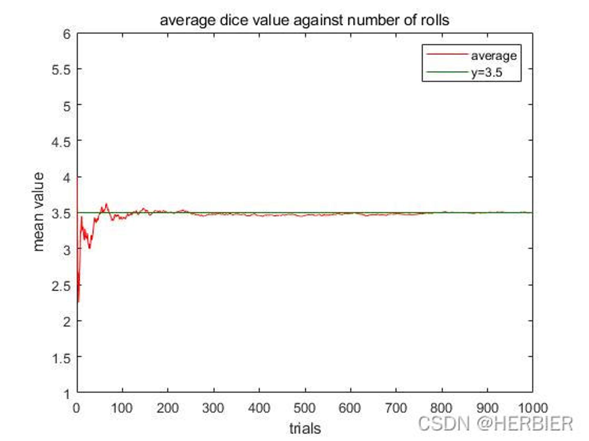

The code is as follows ：

clear all;
clf;
clc;
% Specify how many trials you want to run:
num_trials = 1000;

% Now grab all the dice rolls:
trials = randi(6, [1 num_trials]);

% Plot the results:
figure(1);

% Cumulative sum of the trial results divided by the index gives the average:
plot(cumsum(trials)./(1:num_trials), 'r-');

% Let's put a reference line at 3.5 just for fun (make the color a darker green as well):
hold on;
plot([1 num_trials], [3.5 3.5], 'color', [0 0.5 0]);

% Make it look pretty:
title('average dice value against number of rolls');
xlabel('trials');
ylabel('mean value');
legend('average', 'y=3.5');
axis([0 num_trials 1 6]);

Definition

set up It's independent of each other , Random variable sequence obeying the same distribution , And have mathematical expectations . Before doing The arithmetic mean of these variables , Then for any , Yes

prove

For preliminary knowledge, please refer to previous articles ：

Proof and application of Chebyshev inequality

Definition and properties of expectation and variance

We are looking at the variance of random variables There is , Prove the above results , By expectation 、 Variance and Chebyshev inequality

And from independence

From Chebyshev inequality

In the above formula, make , Immediate

It's a random event . equation （1） indicate , When The probability of this event tends to 1. That is, for any positive number , When Sufficiently large , inequality The probability of establishment is very high . In layman's terms , Sinchin's theorem of large numbers says , For independent identically distributed and mean Random variable of , When When they are very large, their arithmetic averages Probably close to .

For preliminary knowledge, please refer to previous articles ：

Convergence by probability

Xinqin's theorem of large numbers can be described as Weak large number theorem ( Schinchin's law of large Numbers ) Set the random variable Are independent of each other , Obey the same distribution and have mathematical expectations . Then the sequence Converges in probability to , namely

reference

[1] Mao Shisong , Cheng Yiming , Pu Xiaolong . Probability theory and mathematical statistics course （ The second edition ）[M]. Higher Education Press , 2019.

[2] Prosperous and sudden , Xie Shiqian , Pan Chengyi . Probability theory and mathematical statistics [M]. Higher Education Press , 2010.

[3] https://zh.wikipedia.org/wiki/%E5%A4%A7%E6%95%B8%E6%B3%95%E5%89%87