A blog to thoroughly master the theory and practice of particle filter (PF) (matlab version)

Application of particle filter in target tracking ： Particle filtering VS Unscented Kalman filter

Particle filtering — From Bayesian filter to particle filter theory to practice

Originality is not easy. , Please give a compliment to all the big guys passing by

Maneuvering target tracking / Nonlinear filtering / Sensor fusion / Navigation, etc. discuss code connection WX: ZB823618313

Under nonlinear conditions , An important problem in Bayesian filtering is the expression of state distribution and the solution of integral formula , From the analysis in the previous chapter , For general nonlinearity / Non Gaussian system , Analytic solution is not feasible . In numerical approximation , Monte Carlo simulation is one of the most general 、 Effective means , Particle filter is based on Monte Carlo simulation , It approximates the statistical distribution of states by using a set of weighted system state samples . Because Monte Carlo simulation method has wide applicability , The particle filter algorithm can also be applied to general nonlinear systems / Non Gaussian system . however , This filtering method also faces several important problems , Such as effective sampling ( The particle ) How to produce 、 How to transfer particles and how to get the sequential estimation of the system state .

Simple understanding , Particle filter uses a large number of random samples , Using Monte Carlo (MonteCarlo,MC) Simulation technology completes Bayesian recursive filtering (Recursive Bayesian Filter) The process . So this blog starts from Bayesian filtering , A brief introduction to particle filter PF The birth of 、 Application

1、 Problem description

Consider the dynamic model of discrete-time nonlinear systems ,
$$\begin{gathered} x_k=f(x_{k-1},w_{k-1}) \\ {z}_k=h(x_k,v_k)\text{\hspace{1em}(1)} \end{gathered}$$
among $x_k$ by $k$ Target state vector at time ,$z_k$ by $k$ Time measurement vector （ Sensor data ）. The controller is not considered here $u_k$.$w_k$ and $v_k$ They are process noise sequence and measurement noise sequence .$w_k$ and $v_k$ Zero mean Gaussian white noise .

Because the recursive form of Bayesian filtering is based on the posterior probability density of nonlinear systems , So there is no need to assume $w_k$ and $v_k$ Zero mean Gaussian white noise . and KF、EKF、CKF、QKF And so on 、 The measurement noise is Gaussian white noise .

Therefore, particle filter based on Bayesian filter can deal with nonlinear and non Gaussian state estimation problems .

Definition $1$ ~ $k$ Time to state $x_k$ All measured data of are
$$z^k=[z_1^T,z_2^T,\cdots ,z_k^T{]}^T$$

The problem of Bayesian filtering is to calculate the right $k$ Time state $x$ The degree of confidence in the estimate , Therefore, the probability density function is constructed $p(x_k|z^k)$, At a given initial distribution $p(x_0|z_0)=p(x_0)$ after , In theory , The probability density function can be recursively obtained through two steps of prediction and update $p(x_k|z^k)$ Value .

Is there a rudiment of Kalman filter , Ha ha ha , forecast 、 Updates also exist KF in .

2、 Recursive Bayesian filtering

1） forecast

Now suppose $k-1$ The probability density function of time is known , Then by putting Chapman-Kolmogorov Equation application
In dynamic equation (1), Can predict $k$ The prior probability density function of the time state is
$$p(x_k|z^{k-1})=\int p(x_k|x_{k-1})p(k-1|z^{k-1})d{x}_{k-1})\text{\hspace{1em}(2)}$$

actually , The state transition equation is written in the form of probability density ：$$x_k=f(x_{k-1},w_{k-1})\underset{\text{Equivalent}}{=}p(x_k|x_{k-1})$$
type (2) It implicitly assumes that $p(x_k|x_{k-1})=p(x_k|x_{k-1},z^{k-1})$, In fact, this itself is established here , be based on (1) Markov process of formula .

2） to update

In obtaining $p(x_k|z^{k-1})$ On the basis of , combination $k$ New measured value obtained at any time , Based on Bayes formula , You can calculate $k$ The posterior probability density function of the time state :
$$p(x_k|z^k)=\frac{p(z_k|x_k)p(x_k|z^{k-1})}{p(z_k|z^{k-1})}\text{\hspace{1em}(3)}$$
Where the molecule $p(z_k|z^{k-1})$ There is a full probability formula to get
$$p(z_k|z^{k-1})=\int p(z_k|x_k)p(x_k|z^{k-1})d{x}_k\text{\hspace{1em}(4)}$$

I'll just say , The above process is actually the formula deduced by Bayes Houyan , Ha ha ha ha ha

In fact, this is also the updated idea of Kalman filter ： stay $k$ Time is measured $z_k$ after , Use measurements $z_k$ Modified a priori probability , Then the posterior probability of the current time state is obtained . I am just too clever , Ha ha ha

3） be based on $p(x_k|z^k)$ A variety of filters

Tell the truth , You're about status $x_k$ The probability density function of （ Distribution ） All of them , Is it difficult to ascertain their various estimates ？

Here's a reminder for all those who are destined to be , In fact, various filters 、 It is estimated that $p(x_k|z^k)$ The first moment of （$x_k$ Estimation ） And the second moment （ Estimated partners ）.（ Jicao 、 Do not 6）

type (3) This paper describes an example of $k-1$ A posteriori probability density function of time is $k$ The complete process of recursion of time posterior probability density function , Thus, a general expression of the optimal solution of Bayesian estimation is formed . And then through the posterior distribution $p(x_k|z^k)$ Under different criteria $x$ The optimal estimation plan .

Such as minimum mean square error (MMSE) It is estimated that ：
$${\hat{x}}_k=E[x_k|z_k]=\int x_{k}p(x_k|z^k)d{x}_k\text{\hspace{1em}(5)}$$

Maximum posteriori (MAP) It is estimated that ：
$${\hat{x}}_k=\arg \underset{x_k}{\min }p(x_k|z^k)$$

In fact, particle filter is based on Monte Carlo technology 、 The recursive process is realized by a large number of samples .

Did you see this , There is a sense of openness , In fact, the above introduction and derivation are simplified versions , I also added some stupid understanding to it , So there are some misunderstandings 、 For high-level people 、 It is suggested that the classic works are the most useful and rigorous .

3、 Standard particle filter PF

The core idea ： Is to use a group of random samples with corresponding weights ( The particle ) To represent the posterior distribution of States . The basic idea of this method is to select an importance probability density and random sampling from it , Get some random samples with corresponding weights , Adjust the weight based on the state observation . And the position of the particles , These samples are then used to approximate the state posterior distribution , Finally, the weighted sum of these samples is taken as the estimated value of the state . Particle filter is not constrained by the linear and Gaussian assumptions of the system model , The state probability density is described in the form of sample rather than function , So that it does not need too many constraints on the probability distribution of state variables , So it is widely used in nonlinear non Gaussian dynamic systems . For all that , At present, the computation of particle filter is still too large 、 Key problems such as particle degradation need to be solved .

Particle filter is actually based on recursive Bayesian filter MMSE(5) Approximate realization of estimation , The approximate method is Monte Carlo method . Many people should understand why particle filter should be mentioned as Bayesian filter .

Usually, a priori distribution is chosen as the importance density function 、 namely
$$q(x_k|x_{k-1}^{(i)},z_k)=p(x_k|x_{k-1}^{(i)})$$
The importance weight of this function is
$$w_k^{(i)}=w_{k-1}^{(i)}p(z_k|x_k^{(i)})$$
Again $w_k^{(i)}$ Normalization is required to obtain ${\tilde{w}}_k^{(i)}$.

The standard particle filter algorithm steps are ：

Particle filtering PF:
Step 1: according to $p(x_0)$ Sampling to get $N$ A particle $x_0^{(i)}\sim p(x_0)$
For $i=2:N$
  Step 2: The new particle generated from the state transition function is ：$$$x_k^{(i)}\sim p(x_k|x_{k-1}^{(i)})$$
  Step 3: Calculate the importance weight ：$$w_k^{(i)}=w_{k-1}^{(i)}p(z_k|x_k^{(i)})$$
  Step 4: Normalized importance weight ：$${\tilde{w}}_k^{(i)}=\frac{w_k^{(i)}}{{\sum }_{j=1}^N{w}_k^{(j)}}$$
  Step 5: Resample particles using resample method （ Take system resampling as an example ）（ Meet? ）
  Step 6: obtain $k$ A posteriori state estimation of time ：
$$E[{\hat{x}}_k]=\sum _{i=1}^N{x}_k^{(i)}{\tilde{w}}_k^{(i)}$$
End For

Particle filtering PF Algorithm structure diagram

Algorithm ： System resampling （systematic resampling）
For $i=1:N$
  Step 1: Initialize the cumulative probability density function CDF：$c_1=0$
For $i=2:N$
  Step 2: structure CDF: $c_i=c_{i-1}+w_k^{(i)}$
  Step 3: from CDF Start at the bottom of ：$i=1$
  Step 4: Sampling starting point ：$u_1=\mathcal{U}[0,1/N]$
End For
For $j=1:N$
  Step 5: Along the CDF Move : $u_j=u_1+(j-1)/N$
  Step 6: While $u_j>c_i$
      $i=i+1$
     End While
  Step 7: Assignment particle ：$x_k^{(j)}=x_k^{(i)}$
  Step 8: Assignment weight ：$w_k^{(j)}=1/N$
  Step 9: Assign parent ：$i^{(j)}=i$
End For

The idea of resampling is ： Since those with small weights don't work , Then don't . To keep the number of particles constant , They have to be replaced by some new particles . The easiest way to find new particles is to copy a few more heavy particles , As for copying a few ？ Let them distribute among the heavy particles according to their proportion of weight , That is, the boss gets the most , The second one gets more points , And so on . The following is a mathematical description .

In addition to the system resampling method , There are several resampling methods ：
Polynomial resampling
Residual resampling
Random resampling

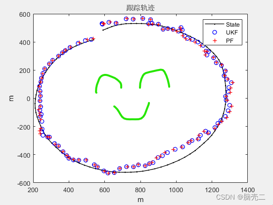
5、 Particle filtering PF In target tracking applications ：

5.1、 Simulation parameters

** One 、 Target model ：CT（ See another blog for details ） **

$$X_{k+1}=\left[\begin{array}{cccc}1& \frac{\sin (\omega T)}{\omega }& 0& -\frac{1-\cos (\omega T)}{\omega }\\ 0& \cos (\omega T)& 0& -\sin (\omega T)\\ 0& \frac{1-\cos (\omega T)}{\omega }& 1& \frac{\sin (\omega T)}{\omega }\\ 0& \sin (\omega T)& 0& \cos (\omega T)\end{array}\right]X_k+\left[\begin{array}{cc}{T}^2/2& 0\\ T& 0\\ 0& T^2/2\\ 0& T\end{array}\right]W_k$$

CV CT See another blog for the specific equation form of the model

Two 、 Measurement model ：2D Active radar
In two dimensions , Radar measurements are range and angle
$$\begin{gathered} r_k^m=r_k+{\tilde{r}}_k \\ {b}_k^m=b_k+{\tilde{b}}_k \end{gathered}$$
among
$$\begin{gathered} r_k=\sqrt{(x_k-x_0{)}^{+}(y_k-y_0{)}^2)} \\ {b}_k={\tan }^{-1}\frac{y_k-y_0}{x_k-x_0} \end{gathered}$$
$[x_0,y_0]$ Is radar coordinates , The general situation is 0. Radar measurement is $z_k=[r_k,b_k{]}^{\prime }$. The radar measurement variance is
$$R_k=\text{cov}(v_k)=\left[\begin{array}{cc}{\sigma }_r^2& 0\\ 0& {\sigma }_b^2\end{array}\right]$$

5.2、 Track and error

6、 Particle filtering PF Standard validation model for

6.1、 Model parameters

State model ：
$$x(k)=f(x(k-1),k)+w(k-1)$$
among
$$f(x((k-1),k)=0.5x(k-1)+2.5x(k-1)/(1+x(k-1{)}^2)+8\cos (1.2k)$$
The measurement equation is ：
$$z(k)=x(k{)}^2/20+v(k)$$

$w(k)$,$v(k)$ The mean is $0$、 The variances are $Q(k)=10$,$R(k)=1$ Gaussian noise of . state $x(k)$ And $x(k-1)$ It is a nonlinear relation , In the observation equation $z(k)$ and x$(k)$ It is also a non-linear relationship .

6.2、 Particle filter based on random resampling PF

6.3、 Particle filter based on polynomial resampling PF

6.4、 Resampling particle filter based on residuals PF

6.5、 Particle filter based on system resampling PF

6.6、 Particle filter based on system resampling PF Code

%%%%%%%%%%%%%%%%%%%%%%%%%%%%%%%%%%%%%%%%%%%%%%%%%%%%%%%%%%%%%%
%%  Particle filter one-dimensional system simulation 
%%%%%%%%%%%%%%%%%%%%%%%%%%%%%%%%%%%%%%%%%%%%%%%%%%%%%%%%%%%%%%
function ParticleFilter_standardmodel
clear all;close all;clc;

randn('seed',1); % In order to ensure that the results of each run are consistent , The seed point of a given random number 
% Initialize related parameters 
T=50;% Number of sampling points 
dt=1;% Sampling period 
Q=10;% Process noise variance 
R=1;% Measure noise variance 
v=sqrt(R)*randn(T,1);% Measuring noise 
w=sqrt(Q)*randn(T,1);% Process noise 
numSamples=100;% Number of particles 
%%%%%%%%%%%%%%%%%%%%%%%%%%%
x0=0.1;% The initial state 
% Generate true states and observations 
X=zeros(T,1);% True state 
Z=zeros(T,1);% Measurement 
X(1,1)=x0;% Real state initialization 
Z(1,1)=(X(1,1)^2)./20+v(1,1);% Observation initialization 
for k=2:T
	% Equation of state 
	X(k,1)=0.5*X(k-1,1)+2.5*X(k-1,1)/(1+X(k-1,1)^2)+8*cos(1.2*k)+w(k-1,1);
	% The observation equation 
	Z(k,1)=(X(k,1).^2)./20+v(k,1);
end
%%%%%%%%%%%%%%%%%%%%%%%%%%%
% Particle filter initialization , It needs to be set to store the filter estimation state , Particle set , Weight and so on 
Xpf=zeros(numSamples,T);% Particle filter estimates the state 
Xparticles=zeros(numSamples,T);% Particle set 
Zpre_pf=zeros(numSamples,T);% Particle filter observation prediction value 
weight=zeros(numSamples,T);% Weight initialization 
% Initial sampling of a given state and observation prediction ：
Xpf(:,1)=x0+sqrt(Q)*randn(numSamples,1);
Zpre_pf(:,1)=Xpf(:,1).^2/20;
% Update and forecast process 
for k=2:T
	% First step ： Particle collection sampling process 
	for i=1:numSamples
		QQ=Q;% Different from Kalman filter , there Q It is not required to be consistent with the process noise variance 
		net=sqrt(QQ)*randn;% there QQ It can be regarded as the radius of the net , Adjustable value 
		Xparticles(i,k)=0.5.*Xpf(i,k-1)+2.5.*Xpf(i,k-1)./(1+Xpf(i,k-1).^2)+8*cos(1.2*k)+net;
	end
	% The second step ： For each particle in the particle set , Calculate its importance weight 
	for i=1:numSamples
		Zpre_pf(i,k)=Xparticles(i,k)^2/20;
		weight(i,k)=exp(-.5*R^(-1)*(Z(k,1)-Zpre_pf(i,k))^2);% The constant term is omitted 
	end
	weight(:,k)=weight(:,k)./sum(weight(:,k));% Normalized weight 
	% The third step ： Resample the particle set according to the weight , Weight set and particle set are one-to-one corresponding 
	% Select a sampling policy 
		outIndex = systematicR(weight(:,k)');
	% Step four ： According to the index obtained by resampling , To pick the corresponding particle , The reconstructed set is the filtered state set 
	% Find the mean of this set of states , Is the final target state 、
	Xpf(:,k)=Xparticles(outIndex,k);
end
% Calculate a posteriori mean estimate 、 Maximum a posteriori estimate and estimated variance 
Xmean_pf=mean(Xpf);% A posteriori mean estimation , And step 4 above , That is, the final state of particle filter estimation 
bins=20;
Xmap_pf=zeros(T,1);
for k=1:T
	[p,pos]=hist(Xpf(:,k,1),bins);
	map=find(p==max(p));
	Xmap_pf(k,1)=pos(map(1));% Maximum posterior estimate 
end
for k=1:T
	Xstd_pf(1,k)=std(Xpf(:,k)-X(k,1));% A posteriori error standard deviation estimation 
end
%%%%%%%%%%%%%%%%%%%%%%%%%%%%%%%%%%%%%%%%%%
% drawing 
figure();clf;% Process noise and measurement noise diagram 
subplot(221);
plot(v);% Measuring noise 
xlabel(' Time ');ylabel(' Measuring noise ');
subplot(222);
plot(w);% Process noise 
xlabel(' Time ');ylabel(' Process noise ');
subplot(223);
plot(X);% True state 
xlabel(' Time ');ylabel(' state X');
subplot(224);
plot(Z);% Observed value 
xlabel(' Time ');ylabel(' observation Z');
%%%%%%%%%%%%%%%%%%%%%%%%%%%%%%%%%%%%%%%%%%%%%
figure();
k=1:dt:T;
plot(k,X,'.-k',k,Xmean_pf,'--ro',k,Xmap_pf,'-.g+','LineWidth',1);% notes ：Xmean_pf Is the result of particle filter 
legend(' True state value of the system ',' A posteriori mean estimation ',' Maximum posterior probability estimation ');
xlabel(' Time ');ylabel(' State estimation ');
%%%%%%%%%%%%%%%%%%%%%%%%%%%%%%%%%%%%%%%%%%%%%%%
figure();
subplot(121);
plot(Xmean_pf,X,'+');% The estimated value of particle filter is consistent with the real state value 1:1 Relationship , Will be symmetrically distributed 
xlabel(' A posteriori mean estimation ');ylabel(' Truth value ');
hold on;
c=-25:1:25;
plot(c,c,'r');% Draw a red symmetry line y=x
hold off;
subplot(122);% The maximum a posteriori estimate is proportional to the true state value 1:1 Relationship , Will be symmetrically distributed 
plot(Xmap_pf,X,'+');
xlabel('Map It is estimated that ');ylabel(' Truth value ');
hold on;
c=-25:25;
plot(c,c,'r');% Draw a red symmetry line y=x
hold off;
%%%%%%%%%%%%%%%%%%%%%%%%%%%%%%%%%%%%%%%%%%%%%%%%%%
% Draw a histogram , This graph is to see the posterior density of the particle set 
domain=zeros(numSamples,1);
range=zeros(numSamples,1);
bins=10;
support=[-20:1:20];
figure();
hold on;% Histogram 
xlabel(' Time ');ylabel(' sample space ');
vect=[0 1];
caxis(vect);
for k=1:T
	% The histogram reflects the distribution of the filtered particle set 
	[range,domain]=hist(Xpf(:,k),support);
	% call waterfall function , Draw the histogram data 
	waterfall(domain,k,range);
end
axis([-20 20 0 T 0 100]);
%%%%%%%%%%%%%%%%%%%%%%%%%%%%%%%%%%%%%%%%%%%%%%%%%%%%
figure();
xlabel(' sample space ');ylabel(' Posterior density ');
k=30;%k=? Indicates the overlapping relationship between the particle distribution and the real state value at the time of viewing 
[range,domain]=hist(Xpf(:,k),support);
plot(domain,range);
% The position of the real state in the sample space , Draw a red line to indicate 
XXX=[X(k,1),X(k,1)];
YYY=[0,max(range)+10];
line(XXX,YYY,'Color','r');
axis([min(domain) max(domain) 0 max(range)+10]);
figure();
k=1:dt:T;
plot(k,Xstd_pf,'-ro','LineWidth',1);
xlabel(' Time ');ylabel(' Standard deviation of state estimation error ');
axis([0,T,0,10]);
%%%%%%%%%%%%%%%%%%%%%%%%%%%%%%%%%%%%


%%%%%%%%%%%%%%%%%%%%%%%%%%%%%%%%%%%%%%%%%%%%%%%%%%%%%%%%%%%
%  The system reacquires the appearance function 
%  Input parameters ：weight Is the weight corresponding to the original data 
%  Output parameters ：outIndex It's based on weight Filter and copy results 
function outIndex = systematicR(weight);
N=length(weight);
N_children=zeros(1,N);
label=zeros(1,N);
label=1:1:N;
s=1/N;
auxw=0;
auxl=0;
li=0;
T=s*rand(1);
j=1;
Q=0;
i=0;
u=rand(1,N);
while (T<1)
    if (Q>T)
        T=T+s;
        N_children(1,li)=N_children(1,li)+1;
    else
        i=fix((N-j+1)*u(1,j))+j;
        auxw=weight(1,i);
        li=label(1,i);
        Q=Q+auxw;
        weight(1,i)=weight(1,j);
        label(1,i)=label(1,j);
        j=j+1;
    end
end
index=1;
for i=1:N
    if (N_children(1,i)>0)
        for j=index:index+N_children(1,i)-1
            outIndex(j) = i;
        end;
    end;
    index= index+N_children(1,i);
end
%%%%%%%%%%%%%%%%%%%%%%%%%%%%%%%%%%%%%%%%%%%%%%%%%%%%%%%

PF Mom Bayesian filtering Part-I、 Monte Carlo method Part-II、 Sequential resampling Part-III

Originality is not easy. , Please give a compliment to all the big guys passing by