Titanic rescued - re exploration of data mining (ideas + source code + results)

Write it at the front ：

I wrote about... When I was just getting started kaggle Prediction of the Titanic's rescue in the competition , As a classic project for many machine learning enthusiasts , After half a year , Have some different feelings , Share with you , It is also a record of the process of stimulating learning .
Welcome to discuss .
（ This article is applicable to friends who have certain foundation , I will try to reduce the language description , Write comments as much as possible ）
Ps: The author's ability is limited , This article is for reference only , Welcome to exchange .

1： Ideas

If it was a vegetable chicken , Now it is a stronger vegetable chicken , For the Titanic project , We need to extract commonalities from features , Find out the general idea of data mining project .
Personal summary is as follows ：

Data mining process ：

1. data fetch
   a. Reading data , And show
   b. Statistical data and various indicators
   c. Clarify the data scale and tasks to be completed
2. Feature understanding and analysis
   a. Single feature analysis , Analyze its impact on the results one by one
   b. Multivariate statistical analysis , Comprehensively consider the impact of various situations
   c. Draw a conclusion by statistical drawing
3. Data cleaning and preprocessing
   a. Fill in missing values
   b. Feature Standardization / normalization
   c . Screen for valuable features
   d. Analyze the correlation between features
4. Build a model
   a. Characteristic data and label preparation
   b. Data set segmentation
   c. Comparison of various modeling algorithms
   d. Integration strategy and other scheme improvements

2 Data reading and statistical analysis

import numpy as np 
import pandas as pd
import matplotlib.pyplot as plt
import seaborn as sns
plt.style.use('fivethirtyeight')
import warnings
warnings.filterwarnings('ignore')
%matplotlib inline

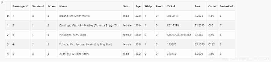
data=pd.read_csv(r'/Titanic/train.csv')
data.head()

# Check for missing values 
data.isnull().sum() #checking for total null values

# Look at the data scale 
data.describe()

# View the rescued proportion 
f,ax=plt.subplots(1,2,figsize=(18,8))
data['Survived'].value_counts().plot.pie(explode=[0,0.1],autopct='%1.1f%%',ax=ax[0],shadow=True)
ax[0].set_title('Survived')
ax[0].set_ylabel('')
sns.countplot('Survived',data=data,ax=ax[1])
ax[1].set_title('Survived')
plt.show()

In the training set 891 Of the passengers , Only about 350 People survived , Only 38.4%

Use different characteristics of the data set to check survival . Like gender , Age , Boarding place, etc ,
First we have to understand the characteristics of the data ！

The data characteristics are divided into ： Continuous and discrete values
Discrete value ： Gender （ male , Woman ） Place of embarkation （S,Q,C）
Continuous value ： Age , Ticket price

data.groupby(['Sex','Survived'])['Survived'].count()

f,ax=plt.subplots(1,2,figsize=(18,8))
data[['Sex','Survived']].groupby(['Sex']).mean().plot.bar(ax=ax[0])
ax[0].set_title('Survived vs Sex')
sns.countplot('Sex',hue='Survived',data=data,ax=ax[1])
ax[1].set_title('Sex:Survived vs Dead')
plt.show()

The survival rate for a woman on a ship is 75% about , And men are 18-19% about .
Pclass --> The relationship between the cabin class and the rescue situation

pd.crosstab(data.Pclass,data.Survived,margins=True).style.background_gradient(cmap='summer_r')

f,ax=plt.subplots(1,2,figsize=(18,8))
data['Pclass'].value_counts().plot.bar(color=['#CD7F32','#FFDF00','#D3D3D3'],ax=ax[0])
ax[0].set_title('Number Of Passengers By Pclass')
ax[0].set_ylabel('Count')
sns.countplot('Pclass',hue='Survived',data=data,ax=ax[1])
ax[1].set_title('Pclass:Survived vs Dead')
plt.show()

pClass1 Survival is 63% about , and pclass2 It's about 48%.
Money is really great ..

Cabin class and gender

pd.crosstab([data.Sex,data.Survived],data.Pclass,margins=True).style.background_gradient(cmap='summer_r')

sns.factorplot('Pclass','Survived',hue='Sex',data=data)
plt.show()

use factorplot It looks more intuitive .

It is easy to infer , from pclass1 Female survival is 95-96%, Such as 94 There is nothing but 3 Women from pclass1 Not rescued .

The obvious thing is , Regardless of pClass, Women are preferred .

therefore Pclass It is also an important feature
Look at your age

print('Oldest Passenger was of:',data['Age'].max(),'Years')
print('Youngest Passenger was of:',data['Age'].min(),'Years')
print('Average Age on the ship:',data['Age'].mean(),'Years')

f,ax=plt.subplots(1,2,figsize=(18,8))
sns.violinplot("Pclass","Age", hue="Survived", data=data,split=True,ax=ax[0])
ax[0].set_title('Pclass and Age vs Survived')
ax[0].set_yticks(range(0,110,10))
sns.violinplot("Sex","Age", hue="Survived", data=data,split=True,ax=ax[1])
ax[1].set_title('Sex and Age vs Survived')
ax[1].set_yticks(range(0,110,10))
plt.show()

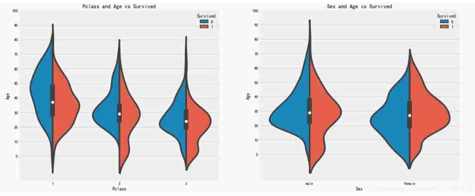
result ：
1）10 The survival rate of children under years old varies with passenegers increase in numbers .

2） Survival is 20-50 The chance of being rescued is higher at the age of .

3） For men , With age , Reduced survival .

Missing value fill

• Average
• Empirical value
• Regression model predicts
• Remove

Age characteristics are 177 A null value . To replace these missing values , Replace with an average

But men and women are different , Divide by address . Simply speaking , Is to find out the average age of women , Find out the average age of men

data['Initial']=0
for i in data:
    data['Initial']=data.Name.str.extract('([A-Za-z]+)\.') 
pd.crosstab(data.Initial,data.Sex).T.style.background_gradient(cmap='summer_r') 

data['Initial'].replace(['Mlle','Mme','Ms','Dr','Major','Lady','Countess','Jonkheer','Col','Rev','Capt','Sir','Don'],['Miss','Miss','Miss','Mr','Mr','Mrs','Mrs','Other','Other','Other','Mr','Mr','Mr'],inplace=True)
data.groupby('Initial')['Age'].mean() #lets check the average age by Initials

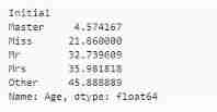
##  Use the mean of each group to fill 
data.loc[(data.Age.isnull())&(data.Initial=='Mr'),'Age']=33
data.loc[(data.Age.isnull())&(data.Initial=='Mrs'),'Age']=36
data.loc[(data.Age.isnull())&(data.Initial=='Master'),'Age']=5
data.loc[(data.Age.isnull())&(data.Initial=='Miss'),'Age']=22
data.loc[(data.Age.isnull())&(data.Initial=='Other'),'Age']=46
data.Age.isnull().any() # Let's see how it's filled 

f,ax=plt.subplots(1,2,figsize=(20,10))
data[data['Survived']==0].Age.plot.hist(ax=ax[0],bins=20,edgecolor='black',color='red')
ax[0].set_title('Survived= 0')
x1=list(range(0,85,5))
ax[0].set_xticks(x1)
data[data['Survived']==1].Age.plot.hist(ax=ax[1],color='green',bins=20,edgecolor='black')
ax[1].set_title('Survived= 1')
x2=list(range(0,85,5))
ax[1].set_xticks(x2)
plt.show()

Conclusion ：
1） Age 5 Saved at the age of , Priority policies for women and children .
2） The oldest passenger was saved （80 year ）.
3） The highest death toll is 30-40 Age group .

sns.factorplot('Pclass','Survived',col='Initial',data=data)
plt.show()

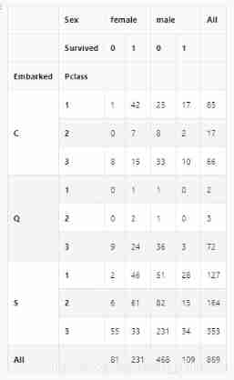
Embarked–> Place of embarkation

pd.crosstab([data.Embarked,data.Pclass],[data.Sex,data.Survived],margins=True).style.background_gradient(cmap='summer_r')

sns.factorplot('Embarked','Survived',data=data)
fig=plt.gcf()
fig.set_size_inches(5,3)
plt.show()

C The highest probability of survival in Hong Kong is 0.55 about , and S The survival rate is the lowest .

f,ax=plt.subplots(2,2,figsize=(20,15))
sns.countplot('Embarked',data=data,ax=ax[0,0])
ax[0,0].set_title('No. Of Passengers Boarded')
sns.countplot('Embarked',hue='Sex',data=data,ax=ax[0,1])
ax[0,1].set_title('Male-Female Split for Embarked')
sns.countplot('Embarked',hue='Survived',data=data,ax=ax[1,0])
ax[1,0].set_title('Embarked vs Survived')
sns.countplot('Embarked',hue='Pclass',data=data,ax=ax[1,1])
ax[1,1].set_title('Embarked vs Pclass')
plt.subplots_adjust(wspace=0.2,hspace=0.5)
plt.show()

Observe :

1） Most people's cabin class is 3.

2）C Our passengers look lucky , Some of them survived .

3）S There are many rich people in the port . The chances of survival are low .

4） port Q Almost 95% All the passengers are poor .

sns.factorplot('Pclass','Survived',hue='Sex',col='Embarked',data=data)
plt.show()

Conclusion ：
1.Pclass1 and Pclass2 The survival rate of women in the study is almost 1
2.Pclass3 People who , Both men and women , The survival rate is impressive
3. port Q Of the people who have the most problems , Because it's all 3 First class
Conclusion ： Money means you can do whatever you want .
Because the port also has missing values , Use the total here to fill in ,

data['Embarked'].fillna('S',inplace=True)
data.Embarked.isnull().any()

sibsip --> The number of brothers and sisters

This characteristic indicates whether a person is alone or with his family .

pd.crosstab([data.SibSp],data.Survived).style.background_gradient(cmap='summer_r')

f,ax=plt.subplots(1,2,figsize=(20,8))
sns.barplot('SibSp','Survived',data=data,ax=ax[0])
ax[0].set_title('SibSp vs Survived')
sns.factorplot('SibSp','Survived',data=data,ax=ax[1])
ax[1].set_title('SibSp vs Survived')
plt.close(2)
plt.show()

pd.crosstab(data.SibSp,data.Pclass).style.background_gradient(cmap='summer_r')

Conclusion ： The survival rate with brothers and sisters is not high .
This is in line with our actual situation .
（ There's a bigger problem , Did you see 5 and 8 The survival rate is 0.. I know ）
And the next one ： Study the number of parents and children

pd.crosstab(data.Parch,data.Pclass).style.background_gradient(cmap='summer_r')

f,ax=plt.subplots(1,2,figsize=(20,8))
sns.barplot('Parch','Survived',data=data,ax=ax[0])
ax[0].set_title('Parch vs Survived')
sns.factorplot('Parch','Survived',data=data,ax=ax[1])
ax[1].set_title('Parch vs Survived')
plt.close(2)
plt.show()

Passengers with parents have a greater chance of survival . however , The extended family is here Pclass3

1-3 People with the highest probability of survival .

Fare- The price of the ticket

print('Highest Fare was:',data['Fare'].max())
print('Lowest Fare was:',data['Fare'].min())
print('Average Fare was:',data['Fare'].mean())

Simply trim ：
Gender ： Compared with men , Women have a high chance of survival .

Pclass： Better survival in first class

Age ： Less than 5-10 The survival rate of children aged 20 is high . Age 15 To 35 Many passengers died between the ages of .

port ： Port and Pclass The relevance is too high

family ： Family size also affects survival

sns.heatmap(data.corr(),annot=True,cmap='RdYlGn',linewidths=0.2) #data.corr()-->correlation matrix
fig=plt.gcf()
fig.set_size_inches(10,8)
plt.show()

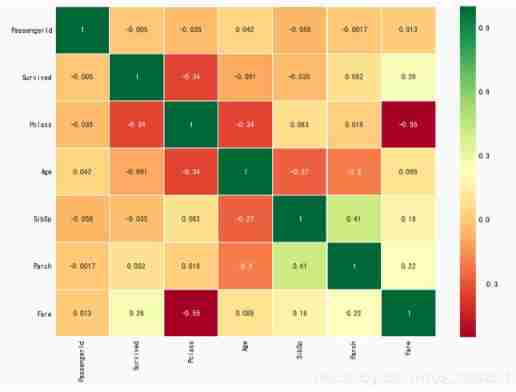
Heat map of characteristic correlation

The first thing to notice is that , Only numerical characteristics are compared
positive correlation ： If features A The increase in leads to the characteristics b An increase in , Then they are positively correlated . value 1 It's a completely positive correlation .
negative correlation ： If features A The increase in leads to the characteristics b The reduction of , There is a negative correlation . value -1 It means completely negative correlation .
If the two characteristics are highly correlated , Or completely relevant , That is, an increase in one will lead to another increase . Both features contain highly similar information ,
In high school mathematics , These two characteristics A and B, And there are A=aB+b, here ,A and B These two characteristics , We only need one .
This is called redundancy ,
Now? , We can see from the picture above . The features we get , No significant correlation .

Feature Engineering and data cleaning

After understanding the relationship of feature correlation , We need to observe , Experience , Or from another Extract information from features to obtain or add new features .

Age characteristics ：

Age is a continuous feature .
There is a problem , such as 30 personal ,30 Age , We can't share 30 Group ,
The problem is simply ： Discrete grouping of continuous values ！
Take this topic for example .
The maximum age of passengers is 80 year , hold 0-80 Divide into 5 Group words ,80/5=16, That is, every 16 Divide into groups .

data['Age_band']=0
data.loc[data['Age']<=16,'Age_band']=0
data.loc[(data['Age']>16)&(data['Age']<=32),'Age_band']=1
data.loc[(data['Age']>32)&(data['Age']<=48),'Age_band']=2
data.loc[(data['Age']>48)&(data['Age']<=64),'Age_band']=3
data.loc[data['Age']>64,'Age_band']=4
data.head(2)

data['Age_band'].value_counts().to_frame().style.background_gradient(cmap='summer')
# Look at the approximate age of each group 

sns.factorplot('Age_band','Survived',data=data,col='Pclass')
plt.show()

You can see from the picture , Survival decreases with age , This is in line with the actual situation ,

Family_size: Total number of families

data['Family_Size']=0
data['Family_Size']=data['Parch']+data['SibSp']#family size
data['Alone']=0
data.loc[data.Family_Size==0,'Alone']=1#Alone

f,ax=plt.subplots(1,2,figsize=(18,6))
sns.factorplot('Family_Size','Survived',data=data,ax=ax[0])
ax[0].set_title('Family_Size vs Survived')
sns.factorplot('Alone','Survived',data=data,ax=ax[1])
ax[1].set_title('Alone vs Survived')
plt.close(2)
plt.close(3)
plt.show()

family_size = 0 signify passeneger It's a person .   
 A person and family 4 More people , The chances of survival are very small .  
 This is an important feature of the model .   

Ticket price

The price of the ticket is also a continuous characteristic , Need to be converted into discrete values
It's used here pandas.qcut

data['Fare_Range']=pd.qcut(data['Fare'],4).cat.codes

data.groupby(['Fare_Range'])['Survived'].mean().to_frame().style.background_gradient(cmap='summer_r')

As mentioned above , We can see clearly that , Ticket prices increase the chances of survival .

data['Fare_cat']=0
data.loc[data['Fare']<=7.91,'Fare_cat']=0
data.loc[(data['Fare']>7.91)&(data['Fare']<=14.454),'Fare_cat']=1
data.loc[(data['Fare']>14.454)&(data['Fare']<=31),'Fare_cat']=2
data.loc[(data['Fare']>31)&(data['Fare']<=513),'Fare_cat']=3
sns.factorplot('Fare_cat','Survived',data=data,hue='Sex')
plt.show()

Conclusion , With fare_cat increase , Increased chance of survival .
About gender , It is easy to modify .0 male 1 Woman
What this shows is ,： We convert strings into numbers .

data['Sex'].replace(['male','female'],[0,1],inplace=True)

There are also some unwanted eigenvalues
name： Unwanted , Don't explain .
Age ： Already grouped .
Ticket number ： Any string , Unable to categorize
The fare ： Use fare_cat features
Bunker number /passengerid --> Cannot be classified

data.drop(['Name','Age','Ticket','Fare','Cabin','Fare_Range','PassengerId'],axis=1,inplace=True)
sns.heatmap(data.corr(),annot=True,cmap='RdYlGn',linewidths=0.2,annot_kws={'size':20})
fig=plt.gcf()
fig.set_size_inches(18,15)
plt.xticks(fontsize=14)
plt.yticks(fontsize=14)
plt.show()

Machine learning modeling

Classical machine learning modeling algorithms include ：
1）logistic Return to

2） Support vector machine （ Linear and radial ）

3） Random forests

4）k- a near neighbor

5） Naive Bayes

6） Decision tree

7） neural network

#importing all the required ML packages
from sklearn.linear_model import LogisticRegression #logistic regression
from sklearn import svm #support vector Machine
from sklearn.ensemble import RandomForestClassifier #Random Forest
from sklearn.neighbors import KNeighborsClassifier #KNN
from sklearn.naive_bayes import GaussianNB #Naive bayes
from sklearn.tree import DecisionTreeClassifier #Decision Tree
from sklearn.model_selection import train_test_split #training and testing data split
from sklearn import metrics #accuracy measure
from sklearn.metrics import confusion_matrix #for confusion matrix

data.head()

train,test=train_test_split(data,test_size=0.3,random_state=0,stratify=data['Survived'])
train_X=train[train.columns[1:]]
train_Y=train[train.columns[:1]]
test_X=test[test.columns[1:]]
test_Y=test[test.columns[:1]]
X=data[data.columns[1:]]
Y=data['Survived']

# Support vector machine --- The kernel function is rbf
model=svm.SVC(kernel='rbf',C=1,gamma=0.1)
model.fit(train_X,train_Y)
prediction1=model.predict(test_X)
print('Accuracy for rbf SVM is ',metrics.accuracy_score(prediction1,test_Y))

# Support vector machine --- The kernel function is linear
model=svm.SVC(kernel='linear',C=0.1,gamma=0.1)
model.fit(train_X,train_Y)
prediction2=model.predict(test_X)
print('Accuracy for linear SVM is',metrics.accuracy_score(prediction2,test_Y))

# Logical regression 
model = LogisticRegression()
model.fit(train_X,train_Y)
prediction3=model.predict(test_X)
print('The accuracy of the Logistic Regression is',metrics.accuracy_score(prediction3,test_Y))

# Decision tree --Decision Tree
model=DecisionTreeClassifier()
model.fit(train_X,train_Y)
prediction4=model.predict(test_X)
print('The accuracy of the Decision Tree is',metrics.accuracy_score(prediction4,test_Y))

#KNN-K-Nearest Neighbors
model=KNeighborsClassifier() 
model.fit(train_X,train_Y)
prediction5=model.predict(test_X)
print('The accuracy of the KNN is',metrics.accuracy_score(prediction5,test_Y))

Now the precision is KNN Changes in the model , change n_neighbours Value attribute to see the effect .
The default value is 5.
Look at the precision in n_neighbours Different results .

a_index=list(range(1,11))
a=pd.Series()
x=[0,1,2,3,4,5,6,7,8,9,10]
for i in list(range(1,11)):
    model=KNeighborsClassifier(n_neighbors=i) 
    model.fit(train_X,train_Y)
    prediction=model.predict(test_X)
    a=a.append(pd.Series(metrics.accuracy_score(prediction,test_Y)))
plt.plot(a_index, a)
plt.xticks(x)
fig=plt.gcf()
fig.set_size_inches(12,6)
plt.show()
print('Accuracies for different values of n are:',a.values,'with the max value as ',a.values.max())

# gaussian 
model=GaussianNB()
model.fit(train_X,train_Y)
prediction6=model.predict(test_X)
print('The accuracy of the NaiveBayes is',metrics.accuracy_score(prediction6,test_Y))

# Random forests 
model=RandomForestClassifier(n_estimators=100)
model.fit(train_X,train_Y)
prediction7=model.predict(test_X)
print('The accuracy of the Random Forests is',metrics.accuracy_score(prediction7,test_Y))

What we get here is all from the training set , But in practice , Is to verify on the test set . The change in accuracy is unknown

Cross validation

Cross validation - Multiple rounds of averaging

1） Cross validation works by first dividing the data set into k-subsets.

2） Suppose we divide the data set into （k＝5） part . We reserve 1 Parts to test , And 4 Training in parts .

3） We continue this process by changing the test part in each iteration and training the algorithm in other parts . Then average the measurement results , The average accuracy of the algorithm is obtained .

This is called cross validation .

from sklearn.model_selection import KFold #for K-fold cross validation
from sklearn.model_selection import cross_val_score #score evaluation
from sklearn.model_selection import cross_val_predict #prediction
kfold = KFold(n_splits=10, random_state=22) # k=10, split the data into 10 equal parts
xyz=[]
accuracy=[]
std=[]
classifiers=['Linear Svm','Radial Svm','Logistic Regression','KNN','Decision Tree','Naive Bayes','Random Forest']
models=[svm.SVC(kernel='linear'),svm.SVC(kernel='rbf'),LogisticRegression(),KNeighborsClassifier(n_neighbors=9),DecisionTreeClassifier(),GaussianNB(),RandomForestClassifier(n_estimators=100)]
for i in models:
    model = i
    cv_result = cross_val_score(model,X,Y, cv = kfold,scoring = "accuracy")
    cv_result=cv_result
    xyz.append(cv_result.mean())
    std.append(cv_result.std())
    accuracy.append(cv_result)
new_models_dataframe2=pd.DataFrame({'CV Mean':xyz,'Std':std},index=classifiers)       
new_models_dataframe2

plt.subplots(figsize=(12,6))
box=pd.DataFrame(accuracy,index=[classifiers])
box.T.boxplot()

new_models_dataframe2['CV Mean'].plot.barh(width=0.8)
plt.title('Average CV Mean Accuracy')
fig=plt.gcf()
fig.set_size_inches(8,5)
plt.show()

Confusion matrix

It gives the number of correct and incorrect classifiers .

f,ax=plt.subplots(3,3,figsize=(12,10))
y_pred = cross_val_predict(svm.SVC(kernel='rbf'),X,Y,cv=10)
sns.heatmap(confusion_matrix(Y,y_pred),ax=ax[0,0],annot=True,fmt='2.0f')
ax[0,0].set_title('Matrix for rbf-SVM')
y_pred = cross_val_predict(svm.SVC(kernel='linear'),X,Y,cv=10)
sns.heatmap(confusion_matrix(Y,y_pred),ax=ax[0,1],annot=True,fmt='2.0f')
ax[0,1].set_title('Matrix for Linear-SVM')
y_pred = cross_val_predict(KNeighborsClassifier(n_neighbors=9),X,Y,cv=10)
sns.heatmap(confusion_matrix(Y,y_pred),ax=ax[0,2],annot=True,fmt='2.0f')
ax[0,2].set_title('Matrix for KNN')
y_pred = cross_val_predict(RandomForestClassifier(n_estimators=100),X,Y,cv=10)
sns.heatmap(confusion_matrix(Y,y_pred),ax=ax[1,0],annot=True,fmt='2.0f')
ax[1,0].set_title('Matrix for Random-Forests')
y_pred = cross_val_predict(LogisticRegression(),X,Y,cv=10)
sns.heatmap(confusion_matrix(Y,y_pred),ax=ax[1,1],annot=True,fmt='2.0f')
ax[1,1].set_title('Matrix for Logistic Regression')
y_pred = cross_val_predict(DecisionTreeClassifier(),X,Y,cv=10)
sns.heatmap(confusion_matrix(Y,y_pred),ax=ax[1,2],annot=True,fmt='2.0f')
ax[1,2].set_title('Matrix for Decision Tree')
y_pred = cross_val_predict(GaussianNB(),X,Y,cv=10)
sns.heatmap(confusion_matrix(Y,y_pred),ax=ax[2,0],annot=True,fmt='2.0f')
ax[2,0].set_title('Matrix for Naive Bayes')
plt.subplots_adjust(hspace=0.2,wspace=0.2)
plt.show()

Explain the confusion matrix ： Look at the first picture

1） The accuracy of the prediction is 491（ Death ）+ 247（ Survive ）, Average CV Accuracy rate is （491+247）/ 891＝82.8%.

2）58 and 95 It's all the wrong amount .
Are you familiar with this picture ？ Remember F1 Coefficient not , Remember the precision and recall ..