当前位置:网站首页>[Deep Learning 21-Day Learning Challenge] 3. Use a self-made dataset - Convolutional Neural Network (CNN) Weather Recognition
[Deep Learning 21-Day Learning Challenge] 3. Use a self-made dataset - Convolutional Neural Network (CNN) Weather Recognition
2022-08-04 06:06:00 【Live up to [email protected]】
活动地址:CSDN21天学习挑战赛
through the first two lessons,Plus a private foundation,The basics of drawing a tiger according to a cat are mastered卷积神经网络-CNNThe basic method of building a model.
之前使用的,All use off-the-shelf datasets,想想,If you really need to apply in the future,肯定需要使用自制数据集来训练模型,刚好k同学啊老师,Such a class was arranged,direct course.
Will learn now总结如下:(The complete code is attached)
1、数据分析
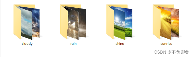
Data downloaded from the teacher,weather_photosThere are four categories under the folder(四个目录):
- cloudy (阴天/多云) :
300张图片 - rain(雨天):
215张图片 - shine (阳光明媚):
253张图片 - sunrise(日出/朝霞):
357张图片
图片都是jpg格式
同时,也可以看到,data picture尺寸各异.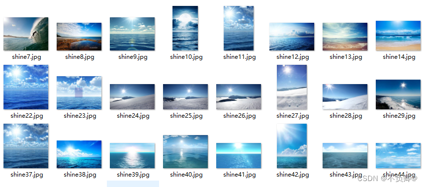
通过分析,可知,在使用数据集之前,At least do it in advance三件事:
- 加载数据
- 统一尺寸
- 分配标签
2、加载数据
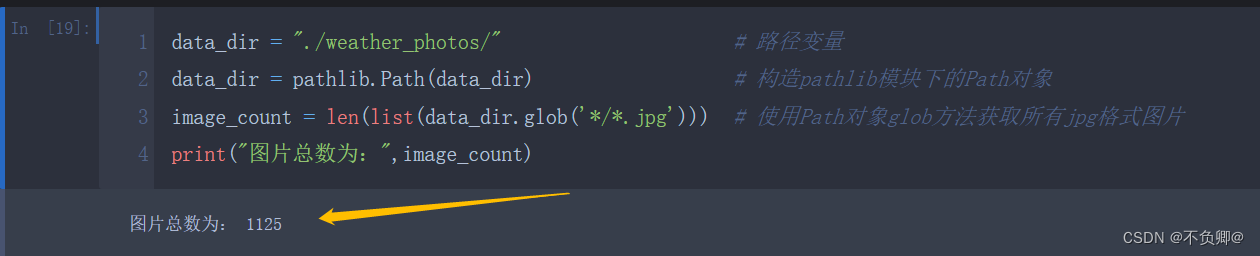
data_dir = "./weather_photos/"                     # 路径变量
data_dir = pathlib.Path(data_dir)                  # 构造pathlib模块下的Path对象
image_count = len(list(data_dir.glob('*/*.jpg')))  # 使用Path对象glob方法获取所有jpg格式图片
print("图片总数为:",image_count)
- I put it in the same directory as the program,所以路径是
"./weather_photos/",You can also base on the actual path,如:data_dir = "D:/datasets/weather_photos/" - 更多用法,Make up for it yourself路径处理库pathlib使用详解
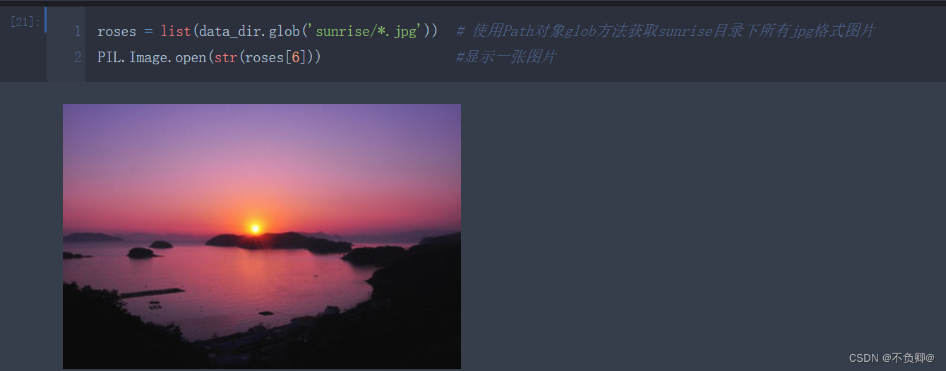
显示图片:
roses = list(data_dir.glob('sunrise/*.jpg'))  # 使用Path对象glob方法获取sunrise目录下所有jpg格式图片
PIL.Image.open(str(roses[6]))                 #显示一张图片
3、数据预处理
3.1、预处理
First define a few important variables:
batch_size = 32
img_height = 180
img_width = 180
- batch_size:深度学习,The data is fed into the neural network in batches,所以,我们来定义,How many pieces of data per batch
- img_height:定义图片高度,之前说过,Self-made data images vary in size,所以,Let's unify the images
- img_width:定义图片宽度,之前说过,Self-made data images vary in size,所以,Let's unify the images
使用: tf.keras.preprocessing.image_dataset_from_directory将文件夹中的数据加载到tf.data.Dataset中,And the loading will disrupt the data at the same time
train_ds = tf.keras.preprocessing.image_dataset_from_directory(
    data_dir,                     # The variables defined above
    validation_split=0.2,         # 保留20%当做测试集
    subset="training",
    seed=123,
    image_size=(img_height, img_width),# The variables defined above
    batch_size=batch_size)             # The variables defined above
参数:
- directory: 数据所在目录.
- validation_split: 0和1之间的数,可保留一部分数据用于验证.如:0.2=20%
- subset:
training或validation.仅在设置validation_split时使用. - image_size:从磁盘读取数据后将其重新调整大小.
- batch_size: 数据批次的大小.默认值:32
后调用class_names将返回以目录同名的类名
class_names = train_ds.class_names
print(class_names)

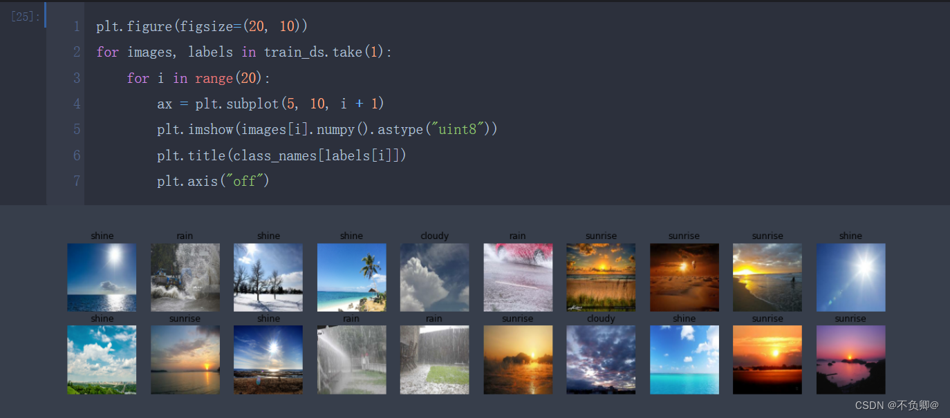
3.2、可视化
plt.figure(figsize=(20, 10))
for images, labels in train_ds.take(1):
    for i in range(20):
        ax = plt.subplot(5, 10, i + 1)
        plt.imshow(images[i].numpy().astype("uint8"))
        plt.title(class_names[labels[i]])
        plt.axis("off")
for image_batch, labels_batch in train_ds:
    print(image_batch.shape)
    print(labels_batch.shape)
    break
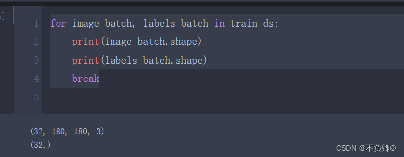
- image_batch: (32, 180, 180, 3) 第一个32is the batch size,180is our modified width and height,3是RGB三个通道
- labels_batch:(32,) 一维,32个标签
3.3、配置数据集
AUTOTUNE = tf.data.AUTOTUNE
train_ds = train_ds.cache().shuffle(1000).prefetch(buffer_size=AUTOTUNE)
val_ds = val_ds.cache().prefetch(buffer_size=AUTOTUNE)  #
- shuffle:数据乱序
- prefetch:Prefetching data speeds up operations
- cache:The dataset is cached in memory,加速
4、构建CNN网络
我们之前学习的,The input dataset shapes are both(28, 28, 1),也就是说,28*28的图像,只有一个颜色通道(灰度)
今天的数据,明显是180*180的图片,并且是RGB三个维度
So we need to define the data shape when declaring the first layer,参数:input_shape
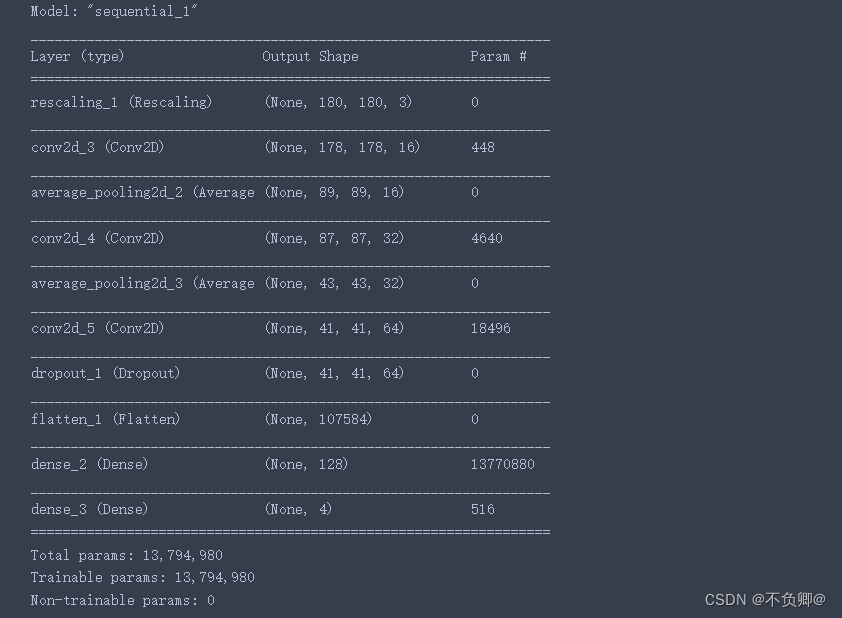
num_classes = 4
model = models.Sequential([
    layers.experimental.preprocessing.Rescaling(1./255, input_shape=(img_height, img_width, 3)),
    layers.Conv2D(16, (3, 3), activation='relu', input_shape=(img_height, img_width, 3)), # 卷积层1,卷积核3*3
    layers.AveragePooling2D((2, 2)),               # 池化层1,2*2采样
    layers.Conv2D(32, (3, 3), activation='relu'),  # 卷积层2,卷积核3*3
    layers.AveragePooling2D((2, 2)),               # 池化层2,2*2采样
    layers.Conv2D(64, (3, 3), activation='relu'),  # 卷积层3,卷积核3*3
    layers.Dropout(0.3),
    layers.Flatten(),                       # Flatten层,连接卷积层与全连接层
    layers.Dense(128, activation='relu'),   # 全连接层,特征进一步提取
    layers.Dense(num_classes)               # 输出层,输出预期结果
])

model.summary()  # 打印网络结构
- 关于model.summary()打印形状,可以看这个
- layers.Dropout(0.4) The role is to prevent overfitting,提高模型的泛化能力.什么是过拟合
- 关于DropoutFor more information on layers, please refer to the article:https://mtyjkh.blog.csdn.net/article/details/115826689
5、配置模型
opt = tf.keras.optimizers.Adam(learning_rate=0.001)
model.compile(optimizer=opt,
              loss=tf.keras.losses.SparseCategoricalCrossentropy(from_logits=True),
              metrics=['accuracy'])
这里没什么好说的,和之前用到的损失函数、优化器一样
使用:learning_rate=0.001is to set the learning rate
- sgd默认为0.01
- adam默认为0.001
6、训练模型
epochs = 10

history = model.fit(
  train_ds,
  validation_data=val_ds,
  epochs=epochs
)
validation_data:Specify test set data
epochs :训练迭代次数
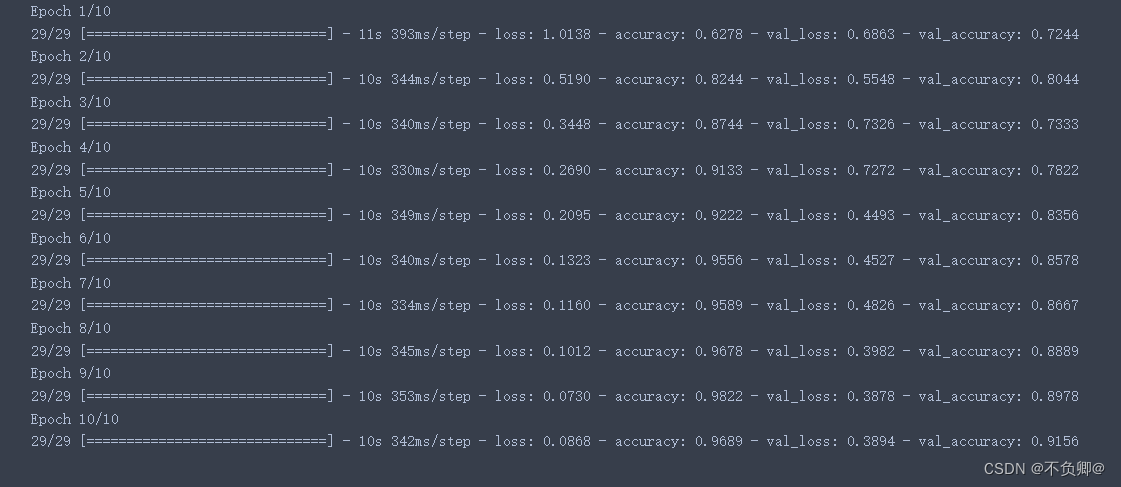
输出说明:loss:训练集损失值
accuracy:训练集准确率
val_loss:测试集损失值
val_accruacy:测试集准确率
7、模型评估
acc = history.history['accuracy']
val_acc = history.history['val_accuracy']

loss = history.history['loss']
val_loss = history.history['val_loss']


epochs_range = range(epochs)

plt.figure(figsize=(12, 4))
plt.subplot(1, 2, 1)
plt.plot(epochs_range, acc, label='Training Accuracy')
plt.plot(epochs_range, val_acc, label='Validation Accuracy')
plt.legend(loc='lower right')
plt.title('Training and Validation Accuracy')

plt.subplot(1, 2, 2)
plt.plot(epochs_range, loss, label='Training Loss')
plt.plot(epochs_range, val_loss, label='Validation Loss')
plt.legend(loc='upper right')
plt.title('Training and Validation Loss')
plt.show()
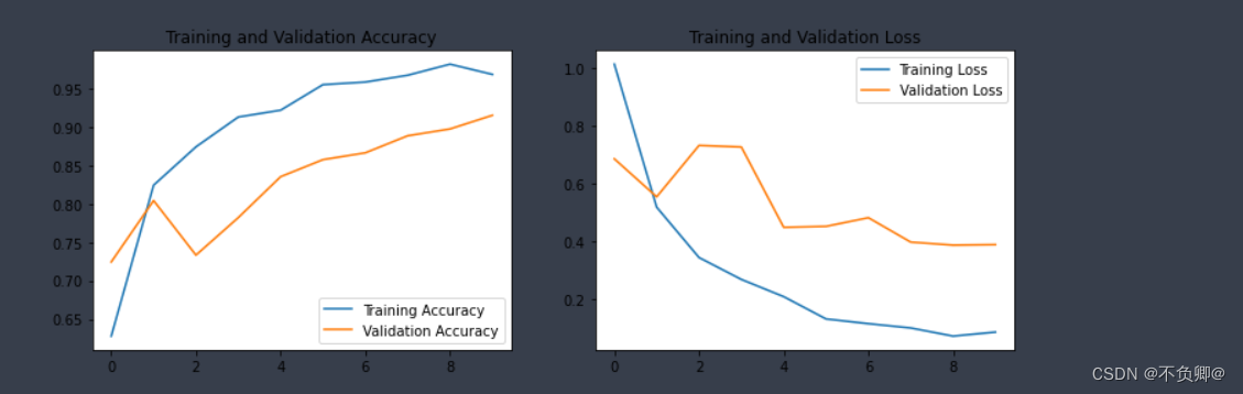
- history :Data returned from training,字典类型,字段:accuracy、loss、val_loss、val_accuracy
8、完整源码
import matplotlib.pyplot as plt
import os,PIL
# 设置随机种子尽可能使结果可以重现
import numpy as np
np.random.seed(1)
# 设置随机种子尽可能使结果可以重现
import tensorflow as tf
tf.random.set_seed(1)
from tensorflow import keras
from tensorflow.keras import layers,models
import pathlib
data_dir = "./weather_photos/"
data_dir = pathlib.Path(data_dir)
image_count = len(list(data_dir.glob('*/*.jpg')))
print("图片总数为:",image_count)
roses = list(data_dir.glob('sunrise/*.jpg'))
PIL.Image.open(str(roses[0]))
batch_size = 32
img_height = 180
img_width = 180
train_ds = tf.keras.preprocessing.image_dataset_from_directory(
    data_dir,
    validation_split=0.2,
    subset="training",
    seed=123,
    image_size=(img_height, img_width),
    batch_size=batch_size)
class_names = train_ds.class_names
print(class_names)
plt.figure(figsize=(20, 10))

val_ds = tf.keras.preprocessing.image_dataset_from_directory(
    data_dir,
    validation_split=0.2,
    subset="validation",
    seed=123,
    image_size=(img_height, img_width),
    batch_size=batch_size)

for images, labels in train_ds.take(1):
    for i in range(20):
        ax = plt.subplot(5, 10, i + 1)

        plt.imshow(images[i].numpy().astype("uint8"))
        plt.title(class_names[labels[i]])

        plt.axis("off")
for image_batch, labels_batch in train_ds:
    print(image_batch.shape)
    print(labels_batch.shape)
    break
# AUTOTUNE = tf.data.AUTOTUNE
AUTOTUNE = tf.data.experimental.AUTOTUNE
train_ds = train_ds.cache().shuffle(1000).prefetch(buffer_size=AUTOTUNE)
val_ds = val_ds.cache().prefetch(buffer_size=AUTOTUNE)
num_classes = 4
model = models.Sequential([
    layers.experimental.preprocessing.Rescaling(1./255, input_shape=(img_height, img_width, 3)),

    layers.Conv2D(16, (3, 3), activation='relu', input_shape=(img_height, img_width, 3)), # 卷积层1,卷积核3*3
    layers.AveragePooling2D((2, 2)),               # 池化层1,2*2采样
    layers.Conv2D(32, (3, 3), activation='relu'),  # 卷积层2,卷积核3*3
    layers.AveragePooling2D((2, 2)),               # 池化层2,2*2采样
    layers.Conv2D(64, (3, 3), activation='relu'),  # 卷积层3,卷积核3*3
    layers.Dropout(0.3),

    layers.Flatten(),                       # Flatten层,连接卷积层与全连接层
    layers.Dense(128, activation='relu'),   # 全连接层,特征进一步提取
    layers.Dense(num_classes)               # 输出层,输出预期结果
])

model.summary()  # 打印网络结构
# 设置优化器
opt = tf.keras.optimizers.Adam(learning_rate=0.001)

model.compile(optimizer=opt,
              loss=tf.keras.losses.SparseCategoricalCrossentropy(from_logits=True),
              metrics=['accuracy'])
epochs = 10

history = model.fit(
  train_ds,
  validation_data=val_ds,
  epochs=epochs
)
acc = history.history['accuracy']
val_acc = history.history['val_accuracy']

loss = history.history['loss']
val_loss = history.history['val_loss']

epochs_range = range(epochs)

plt.figure(figsize=(12, 4))
plt.subplot(1, 2, 1)
plt.plot(epochs_range, acc, label='Training Accuracy')
plt.plot(epochs_range, val_acc, label='Validation Accuracy')
plt.legend(loc='lower right')
plt.title('Training and Validation Accuracy')

plt.subplot(1, 2, 2)
plt.plot(epochs_range, loss, label='Training Loss')
plt.plot(epochs_range, val_loss, label='Validation Loss')
plt.legend(loc='upper right')
plt.title('Training and Validation Loss')
plt.show()
学习日记
1,学习知识点
a、Basic usage of homemade datasets
b、pathlib模块的基本使用
c、tf.keras.preprocessing.image_dataset_from_directory基本使用方法
2,学习遇到的问题
继续啃西瓜书,恶补基础
版权声明
本文为[Live up to [email protected]]所创,转载请带上原文链接,感谢
https://yzsam.com/2022/216/202208040525326846.html
边栏推荐
- 安装dlib踩坑记录,报错:WARNING: pip is configured with locations that require TLS/SSL
- EPSON RC+ 7.0 使用记录一
- 剑指 Offer 20226/30
- CTFshow—Web入门—信息(1-8)
- 剑指 Offer 2022/7/8
- 【树 图 科 技 头 条】2022年6月27日 星期一 今年ETH2.0无望
- TensorFlow2 study notes: 6. Overfitting and underfitting, and their mitigation solutions
- RecyclerView的用法
- flink-sql所有数据类型
- WARNING: sql version 9.2, server version 11.0.Some psql features might not work.
猜你喜欢
随机推荐
Jupyter Notebook installed library;ModuleNotFoundError: No module named 'plotly' solution.
线性回归简介01---API使用案例
Postgresql 快照
多项式回归(PolynomialFeatures)
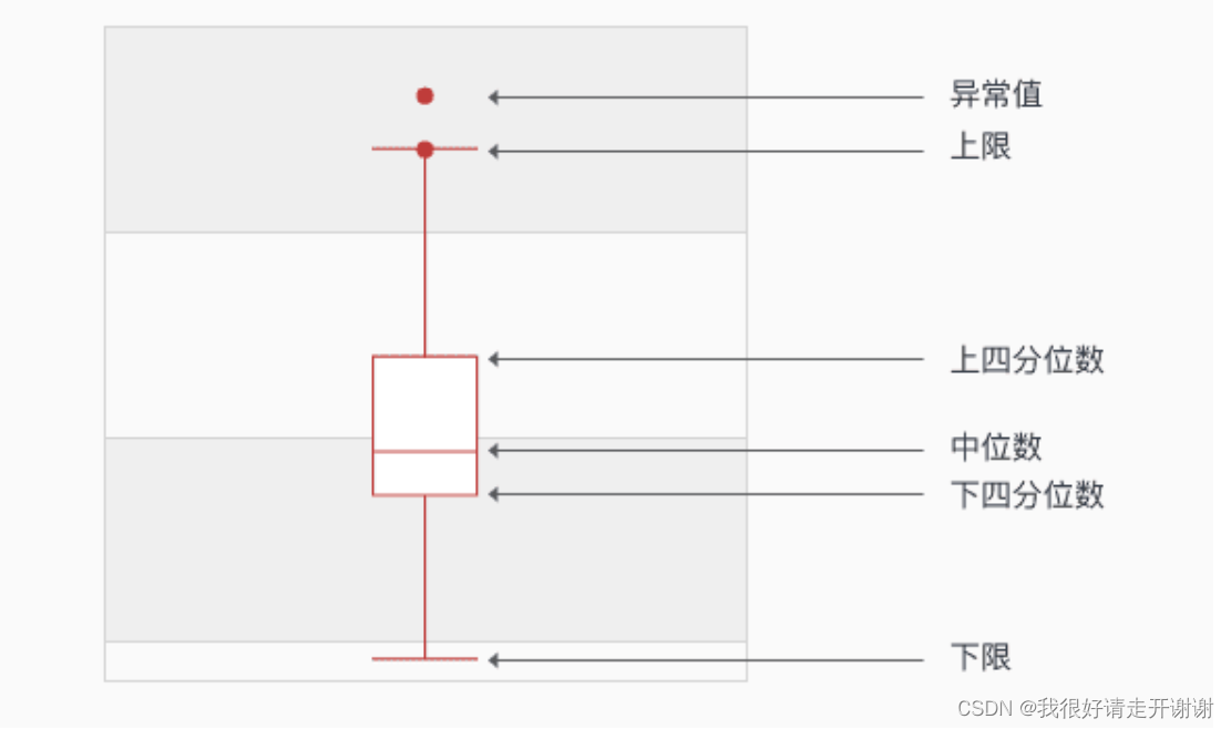
彻底搞懂箱形图分析
flink-sql所有数据类型
The pipeline mechanism in sklearn
记一次flink程序优化
自动化运维工具Ansible(7)roles
数据库根据提纲复习
自动化运维工具Ansible(2)ad-hoc
Learning curve learning_curve function in sklearn
MySql--存储引擎以及索引
二月、三月校招面试复盘总结(一)
【深度学习21天学习挑战赛】3、使用自制数据集——卷积神经网络(CNN)天气识别
TensorFlow2学习笔记:8、tf.keras实现线性回归,Income数据集:受教育年限与收入数据集
Androd Day02
剑指 Offer 2022/7/1
Android connects to mysql database using okhttp
【go语言入门笔记】13、 结构体(struct)