SQL tuning guide notes 9:joins

This paper is about SQL Tuning Guide The first 9 Chapter “Join” The notes .

Important basic concepts

• join condition
  A condition that compares two row sources using an expression. The database combines pairs of rows, each containing one row from each row source, for which the join condition evaluates to true.
  Add conditions
  Use an expression to compare the conditions of two row sources . The database combines pairs of rows , Each row contains one row from each row source , For these lines , The calculation result of the connection condition is true .

• left deep join tree
  A join tree in which the left input of every join is the result of a previous join.
  A connection tree , The left input of each connection is the result of the previous connection .

• right deep join tree
  A join tree in which the right input of every join is the result of a previous join, and the left child of every internal node of a join tree is a table.
  A connection tree , The right input of each connection is the result of the previous connection , The left child of each internal node of the connection tree is a table .

• left table
  In an outer join, the table specified on the left side of the OUTER JOIN keywords (in ANSI SQL syntax).
  In the external connection , stay OUTER JOIN The table specified on the left of the keyword （ stay ANSI SQL In the syntax ）.

• right table
  In an outer join, the table specified on the right side of the OUTER JOIN keywords (in ANSI SQL syntax).
  In the external connection , stay OUTER JOIN The table specified to the right of the keyword （ stay ANSI SQL In the syntax ）.

Oracle The database provides several optimizations for joining rowsets .

• partition-wise join
  Intelligent partition connection

9.1 About Joins

The join will come from exactly two row sources （ For example, tables or views ） The outputs of are grouped together , And return a row source . The row source returned is the dataset .

Connection is characterized by SQL Of the statement WHERE（ Not ANSI） or FROM … JOIN (ANSI) Multiple tables in clause . as long as FROM There are multiple tables in the clause ,Oracle The database will perform the join .

Join conditions use expressions to compare two row sources . Join conditions define the relationships between tables . If the statement does not specify a join condition , Then the database performs Cartesian join , Match each row in one table to each row in another table .

9.1.1 Join Trees

Usually , The connection tree is represented as an inverted tree structure .

As shown in the figure below ,table1 It is the left table ,table2 It's the right table . The optimizer processes connections from left to right . for example , If this figure depicts a nested loop connection , be table1 It's an external circulation , and table2 Internal circulation .

The input of the connection can be the result set of the previous connection . If the right child node of each internal node of the connection tree is a table , Then the tree is a left deep join tree , As shown in the following example . Most join trees are left deep join .

If the left child node of each internal node of the connection tree is a table , Then the tree is called right deep join tree , As shown in the figure below .

If the left or right child node of the internal node of the connection tree can be the connection node , The tree is called a dense join tree . In the following example ,table4 Is the right child node of the connection node ,table1 Is the left child node of the connection node ,table2 Is the left child node of the connection node .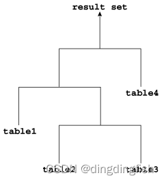

In another variant , Both inputs of the connection are the result of the previous connection .

9.1.2 How the Optimizer Executes Join Statements

Database connection pairs of row sources . When FROM When more than one table exists in the clause , The optimizer must determine the most efficient join operation for each pair .

The optimizer must make the relevant decisions shown in the following table .

• Access path
  For simple statements , The optimizer must select an access path to retrieve data from each table in the join statement . for example , The optimizer may choose between a full table scan or an index scan .
• Connection method
  To join each pair of row sources ,Oracle The database must decide how to proceed . “ how ” Connection method . A possible join method is a nested loop 、 Sort merge and hash join . Cartesian connection requires one of the above connection methods . Each method of connection has a particular case that is more appropriate than the others .
• Connection type
  The connection condition determines the connection type . for example , The inner join retrieves only the rows that match the join criteria . The outer join retrieves rows that do not match the join criteria .
• Connection sequence
  To execute a statement that joins more than two tables ,Oracle The database connects two tables , Then connect the generated row source to the next table . This process continues until all tables are added to the results . for example , The database connects two tables , Then connect the results to the third table , Then connect this result to the fourth table , And so on .

9.1.3 How the Optimizer Chooses Execution Plans for Joins

When determining the connection sequence and method , The goal of the optimizer is to reduce the number of rows as early as possible , So that throughout SQL Less work during statement execution .

The optimizer depends on the possible connection order 、 Connection methods and available access paths generate a set of execution plans . The optimizer then estimates the cost of each plan and selects the one with the lowest cost . When choosing an execution plan , The optimizer considers the following factors ：

• The optimizer first determines whether joining two or more tables will result in a row source containing at most one row .
  The optimizer based on the UNIQUE and PRIMARY KEY Constraints identify this situation . If this is the case , Then the optimizer will put these tables at the top of the join order . The optimizer then optimizes the joins of the remaining table sets .

• For connection statements with outer connection conditions , Tables with outer join operators usually follow another table in the condition in the join order .
  Usually , The optimizer does not consider the order of connections that violate this criterion , Although the optimizer may override this sort condition in some cases . Again , When a subquery has been converted to a de join or semi join , Tables from subqueries must follow those in the external query block to which they are connected or associated . however , Hash anti join and semi join can override this sort condition in some cases .

The optimizer calculates the estimated I/O and CPU To estimate the cost of the query plan . these I/O There are specific costs associated with it ： Single block I/O Cost and multiple pieces I/O Another cost of . Besides , Different functions and expressions have related CPU cost . The optimizer uses these metrics to determine the total cost of the query plan . These metrics can be affected by many initialization parameters and session settings at compile time , for example DB_FILE_MULTI_BLOCK_READ_COUNT Set up 、 System statistics, etc .

for example , The optimizer estimates costs by ：

• The cost of nested loop joins depends on the cost of reading each selected row of the external table and each matching row of the internal table into memory . The optimizer uses statistics from the data dictionary to estimate these costs .
• The cost of sorting merge connections depends largely on the cost of reading all sources into memory and sorting them .
• The cost of a hash connection depends largely on the cost of building a hash table on one input side of the connection and detecting it with rows from the other side of the connection .

conceptually , The optimizer builds a matrix linking the order and method and the costs associated with each . for example , The optimizer must determine how best to join in the query date_dim and lineorder surface . The following table shows possible changes in methods and orders , And the cost of each . In this example , With date_dim,lineorder Sequential connection Has the lowest nested loop cost .

9.2 Join Methods

The connection method is a mechanism for connecting two row sources .

According to statistics , The optimizer chooses the method with the lowest estimated cost . Pictured 9-5 Shown , Each connection method has two children ： drive （ Also known as external ） Row source and drive target （ Also called internal ） Row source .

9.2.1 Nested Loops Joins

Nested loops connect external data sets to internal data sets .

For each row in the external dataset that matches a single table predicate , The database retrieves all rows in the internal dataset that satisfy the join predicate . If the index is available , Then the database can use it to access the information provided by rowid Set internal data .

9.2.1.1 When the Optimizer Considers Nested Loops Joins

When the database is connected to a small subset of data 、 The database connects to a large amount of data and the optimizer mode is set to FIRST_ROWS, Or when the join condition has a valid method to access the internal table （ If the inner table is indexed ）, Nested loop joins are very useful .

Be careful ： The expected number of rows to join is the driver of the optimizer's decision , Not the size of the underlying table . for example , A query may join two tables , Each watch has 10 Billion rows , But because of the filter , The optimizer expects each data set to have 5 That's ok .

Generally speaking , Nested loop join works best on small tables with indexes on join conditions . If the row source has only one row , For example, perform an equality search on the primary key value （ for example ,WHERE employee_id=101）, Then the connection is a simple search . The optimizer always tries to put the smallest row source first , Make it a driving table .

Various factors enter the optimizer's decision to use nested loops . for example , The database can read several rows from external row sources in batches . Based on the number of rows retrieved , The optimizer can select nested loops or hash connections to internal row sources . for example , If the query connects departments to the drive table employees, And if the predicate specifies employees.last_name The value in , The database may read last_name Enough entries in the index to determine if the internal threshold is exceeded . If the threshold is not passed , Then the optimizer selects nested loop connection for departments , If you pass the threshold , Then the database performs a hash connection , This means reading the rest of the staff , Hash it into memory , Then join the Department .（ This is actually adaptive plan）

If the access path of the inner loop does not depend on the outer loop , Then the result can be a Cartesian product ： For each iteration of the outer loop , Inner loops all produce the same rowset . To avoid this problem , Please use other connection methods to connect two independent row sources .

9.2.1.2 How Nested Loops Joins Work

conceptually , A nested loop is equivalent to two nested for loop .

for example , If the query connects employees and departments , Then the nested loop in the pseudo code may be ：

FOR erow IN (select * from employees where X=Y) LOOP
  FOR drow IN (select * from departments where erow is matched) LOOP
    output values from erow and drow
  END LOOP
END LOOP

Each line of the outer loop executes an inner loop . employees Table is “ external ” Data sets , Because it's on the outside for In circulation . External tables are sometimes called drive tables . Department table is “ Inside ” Data sets , Because it's inside for In circulation .

Nested loop joins involve the following basic steps ：

1. The optimizer determines the drive row source and specifies it as an outer loop .
   The outer loop generates a set of rows to drive the join condition . The row source can be an index scan 、 A table accessed by a full table scan or any other operation that generates rows .
   The number of iterations of the inner loop depends on the number of rows retrieved in the outer loop . for example , If... Is retrieved from an external table 10 That's ok , Then the database must execute in the internal table 10 Search times . If... Is retrieved from an external table 10,000,000 That's ok , The database must execute in the inner table 10,000,000 Search times .
2. The optimizer specifies another row source as an internal loop .
   In the execution plan , The outer circulation occurs before the inner circulation , as follows ：

NESTED LOOPS 
  outer_loop
  inner_loop 

3. For every client fetch request , The basic process is as follows ：
   a. Get a row from an external row source
   b. Probe the internal row source to find rows that match the predicate condition
   c. Repeat the above steps , until fetch Request to get all rows

Sometimes , Database pair rowid Sort for more efficient buffer access patterns .

9.2.1.3 Nested Nested Loops

The outer loop of a nested loop itself can be a row source generated by different nested loops .

The database can nest two or more external loops , To connect as many tables as needed . Each loop is a data access method . The following template shows how the database iterates through three nested loops ：

SELECT STATEMENT
  NESTED LOOPS 3
    NESTED LOOPS 2          - Row source becomes OUTER LOOP 3.1
      NESTED LOOPS 1        - Row source becomes OUTER LOOP 2.1
        OUTER LOOP 1.1
        INNER LOOP 1.2  
      INNER LOOP 2.2
    INNER LOOP 3.2

for example ：

set pages 9999
SELECT /*+ ORDERED USE_NL(d) */ e.last_name, e.first_name, d.department_name
FROM   employees e, departments d
WHERE  e.department_id=d.department_id
AND    e.last_name like 'A%';

select * from table(dbms_xplan.display_cursor);

-----------------------------------------------------------------------------------------------------
| Id  | Operation                             | Name        | Rows  | Bytes | Cost (%CPU)| Time     |
-----------------------------------------------------------------------------------------------------
|   0 | SELECT STATEMENT                      |             |       |       |     5 (100)|          |
|   1 |  NESTED LOOPS                         |             |     3 |   102 |     5   (0)| 00:00:01 |
|   2 |   NESTED LOOPS                        |             |     3 |   102 |     5   (0)| 00:00:01 |
|   3 |    TABLE ACCESS BY INDEX ROWID BATCHED| EMPLOYEES   |     3 |    54 |     2   (0)| 00:00:01 |
|*  4 |     INDEX RANGE SCAN                  | EMP_NAME_IX |     3 |       |     1   (0)| 00:00:01 |
|*  5 |    INDEX UNIQUE SCAN                  | DEPT_ID_PK  |     1 |       |     0   (0)|          |
|   6 |   TABLE ACCESS BY INDEX ROWID         | DEPARTMENTS |     1 |    16 |     1   (0)| 00:00:01 |
-----------------------------------------------------------------------------------------------------
 
Predicate Information (identified by operation id):
---------------------------------------------------
 
   4 - access("E"."LAST_NAME" LIKE 'A%')
       filter("E"."LAST_NAME" LIKE 'A%')
   5 - access("E"."DEPARTMENT_ID"="D"."DEPARTMENT_ID")

The example in the original text is very detailed , This will not be repeated .

9.2.1.4 Current Implementation for Nested Loops Joins

Oracle database 11g A new implementation of nested loops is introduced , Can reduce physical I/O The overall delay .

When the index or table block is not in the buffer cache and the connection needs to be processed , It needs physics I/O. The database can batch process multiple physical I/O request , And use vectors I/O（ Array ） Instead of dealing with one at a time . The database will be a set of rowids Sent to the operating system that performs the read .

9.2.1.5 Original Implementation for Nested Loops Joins

Although it's very detailed , But I didn't quite understand the difference between the two .

9.2.1.6 Nested Loops Controls

You can add USE_NL Prompt to instruct the optimizer to join each specified table to another row source with nested loop joins , Use the specified table as the inner table .

Relevant tips USE_NL_WITH_INDEX(table index) The prompt instructs the optimizer to use the specified table as the inner table , Connect the specified table to another row source through nested loop joins . The index is optional . If the index is not specified , The nested loop join uses the index with at least one join predicate as the index key .

To force nested loop joins using departments as internal tables , Please add USE_NL Tips , As shown in the following query ：

-- The ORDERED hint causes Oracle to join tables in the order in which they appear in the FROM clause.

SELECT /*+ ORDERED USE_NL(d) */ e.last_name, d.department_name
FROM   employees e, departments d
WHERE  e.department_id=d.department_id;

9.2.2 Hash Joins

The database uses hash connections to connect to larger datasets .

The optimizer uses the smaller one of the two data sets to build a hash table on the connection key in memory , Use a deterministic hash function to specify where each row is stored in the hash table . Then the database scans a larger data set , Probe the hash table to find the rows that meet the connection conditions .

9.2.2.1 When the Optimizer Considers Hash Joins

Generally speaking , When you need to connect a large amount of data （ Or a large part of the small table needs to be connected ） when , The optimizer will consider using hash joins , This connection is an equivalent connection .

When smaller datasets fit in memory , Hash connections are the most cost-effective . under these circumstances , The cost is limited to one read of two data sets .

Because the hash table is in PGA in , therefore Oracle The database can access rows without locking them . This technique reduces logic by avoiding the need to repeatedly lock and read blocks in the database buffer cache I/O.

If the data set is not suitable for memory , Then the database will partition the row source , And the connection will be made partition by partition . This can use a lot of sort area memory and temporary table space I/O. This is still the most cost-effective method , Especially when the database uses a parallel query server .

9.2.2.2 How Hash Joins Work

The hash algorithm uses a set of inputs and applies a deterministic hash function to generate random hash values .

In hash join , The input value is the connection key . The output value is the index in the array （ Slot ）, It's a hash table .

9.2.2.2.1 Hash Tables

To illustrate the hash table , Suppose that the database is linked to... In the connection between departments and employees hr.departments Hash . The join key column is department_id.

Before department table 5 The line is as follows ：

SQL> select * from departments where rownum < 6;
 
DEPARTMENT_ID DEPARTMENT_NAME                MANAGER_ID LOCATION_ID
------------- ------------------------------ ---------- -----------
           10 Administration                        200        1700
           20 Marketing                             201        1800
           30 Purchasing                            114        1700
           40 Human Resources                       203        2400
           50 Shipping                              121        1500

The database applies a hash function to each department in the table ID, Generate a hash value for each department . For this example , The hash table has 5 Slot （ It may have more or less ）. because n yes 5, So the range of possible hash values is 1 To 5. The hash function might be a department ID Generate the following values ：

f(10) = 4
f(20) = 1
f(30) = 4
f(40) = 2
f(50) = 5

Please note that , The hash function happens to be a department 10 and 30 Generate the same hash value 4. This is called a hash conflict . under these circumstances , The database uses linked lists to link departments 10 and 30 Records of are placed in the same slot . conceptually , The hash table is as follows ：

1    20,Marketing,201,1800
2    40,Human Resources,203,2400
3
4    10,Administration,200,1700 -> 30,Purchasing,114,1700
5    50,Shipping,121,1500

From the above results , Even hash conflicts don't matter , Because additional values are stored .

9.2.2.2.2 Hash Join: Basic Steps

The optimizer uses smaller data sources to build hash tables on in memory join keys , Then scan the larger table for connected rows .

The basic steps are as follows ：

1. Database for smaller datasets （ It is called build table ） Perform a full scan , Then apply the hash function to the join key in each row , In the PGA Build hash table in .
   In pseudocode , The algorithm might look like this ：

FOR small_table_row IN (SELECT * FROM small_table)
LOOP
  slot_number := HASH(small_table_row.join_key);
  INSERT_HASH_TABLE(slot_number,small_table_row);
END LOOP;

2. The database uses the lowest cost access mechanism to probe the second data set , It is called probe table .
   Usually , The database performs a full table scan on smaller and larger datasets . The algorithm in the pseudo code might look like this ：

FOR large_table_row IN (SELECT * FROM large_table)
LOOP
   slot_number := HASH(large_table_row.join_key);
   small_table_row = LOOKUP_HASH_TABLE(slot_number,large_table_row.join_key);
   IF small_table_row FOUND
   THEN
      output small_table_row + large_table_row;
   END IF;
END LOOP;

If there are multiple rows in the hash table slot , Then the database traverses the linked list of rows , Check every line . for example , If the Department 30 Hash to slot 4, Then the database checks each row , Until I find 30.

for example ：

SELECT o.customer_id, l.unit_price * l.quantity
FROM   orders o, order_items l
WHERE  l.order_id = o.order_id;

--------------------------------------------------------------------------
| Id  | Operation            |  Name        | Rows  | Bytes | Cost (%CPU)|
--------------------------------------------------------------------------
|   0 | SELECT STATEMENT     |              |   665 | 13300 |     8  (25)|
|*  1 |  HASH JOIN           |              |   665 | 13300 |     8  (25)|
|   2 |   TABLE ACCESS FULL  | ORDERS       |   105 |   840 |     4  (25)|
|   3 |   TABLE ACCESS FULL  | ORDER_ITEMS  |   665 |  7980 |     4  (25)|
--------------------------------------------------------------------------

Predicate Information (identified by operation id):
---------------------------------------------------
   1 - access("L"."ORDER_ID"="O"."ORDER_ID")

Because relative to big 6 Times order_items surface ,orders The watch is very small , So the database hashes the order . In hash join , The dataset of the build table always appears at the top of the action list （ step 2）. Steps in 3 in , The database will be used later for larger order_items Perform a full scan , Probe the hash table of each row .

9.2.2.3 How Hash Joins Work When the Hash Table Does Not Fit in the PGA

When hash tables do not fit perfectly PGA when , Databases must use different technologies . under these circumstances , The database uses a temporary space to hold parts of the hash table （ Zoning ）, Sometimes it also includes sections that probe the larger tables of the hash table .

The basic process is as follows ：

1. The database performs a full scan of smaller datasets , And then in PGA And build a hash bucket array on disk .
   When PGA When the hash area is full , The database will find the largest partition in the hash table and write it to the temporary space on the disk . The database stores any new rows belonging to the disk partition on disk , And store all other rows in PGA in . therefore , Part of the hash table is in memory , Part of it is on disk .
2. The database starts the first round of reading other data sets .
3. The database reads the temporary partitions on each disk one by one
4. The database connects each partition row to the row in the corresponding temporary disk partition .

9.2.2.4 Hash Join Controls

USE_HASH The prompt instructs the optimizer to use hash joins when joining two tables together .

9.2.3 Sort Merge Joins

Sort merge join is a variant of nested loop join .

If two datasets in the connection have not been sorted , The database sorts them . These are SORT JOIN operation . For each row in the first dataset , The database detects the matching rows of the second dataset and joins them , Its starting position is based on the match in the previous iteration . This is a MERGE JOIN operation .

9.2.3.1 When the Optimizer Considers Sort Merge Joins

A hash connection requires a hash table and a probe into the table , The sort merge join requires two sorts .

When any of the following conditions is met , The optimizer may choose to sort merge joins instead of hash joins to join large amounts of data ：

• The join condition between two tables is not equivalent , That is to use <、<=、>、>= Wait for unequal conditions .
  Compared with sort merge , Hash join requires equality condition .

• Because other operations require sorting , The optimizer finds it cheaper to use sort merge .
  If there is an index , The database can avoid sorting the first dataset . however , Whatever the index , The database always sorts the second data set （ Why? ？）.

Compared with nested loop connection , Sort merge has the same advantages as hash join ： Database access PGA Instead of SGA, Reduce logic by avoiding repeated locking and the need to read blocks from the database buffer cache I/O. Generally speaking , Hash joins perform better than sort merge joins , Because sorting is expensive . however , Sort merge joins offer the following advantages over hash joins ：

• After the initial sort , Optimize consolidation phase , This results in faster generation of output lines .
• When the hash table cannot be completely put into memory , Sort merges can be more cost-effective than hash joins .
  A hash join with insufficient memory needs to copy the hash table and other data sets to disk . under these circumstances , The database may have to be read from disk multiple times . In sort merge , If memory cannot hold two data sets , Then the database writes them all to disk , But read each data set no more than once .

9.2.3.2 How Sort Merge Joins Work

Same as nested loop connection , Sort merge join reads two datasets , But sort them before they are sorted .

For each row in the first dataset , The database finds a starting row in the second dataset , Then read the second data set , Until a mismatched row is found . In pseudocode , An advanced algorithm for sorting and merging might look like this ：

READ data_set_1 SORT BY JOIN KEY TO temp_ds1
READ data_set_2 SORT BY JOIN KEY TO temp_ds2
 
READ ds1_row FROM temp_ds1
READ ds2_row FROM temp_ds2

WHILE NOT eof ON temp_ds1,temp_ds2
LOOP
    IF ( temp_ds1.key = temp_ds2.key ) OUTPUT JOIN ds1_row,ds2_row
    ELSIF ( temp_ds1.key <= temp_ds2.key ) READ ds1_row FROM temp_ds1
    ELSIF ( temp_ds1.key => temp_ds2.key ) READ ds2_row FROM temp_ds2
END LOOP

In fact, the premise of the above algorithm , Or equivalent query .

Let's take an example , In this case , Peripheral strap index , There is no need to reorder ：

set pages 9999
SELECT e.employee_id, e.last_name, e.first_name, e.department_id, 
       d.department_name
FROM   employees e, departments d
WHERE  e.department_id = d.department_id
ORDER BY department_id;


select * from table(dbms_xplan.display_cursor);

--------------------------------------------------------------------------------------------
| Id  | Operation                    | Name        | Rows  | Bytes | Cost (%CPU)| Time     |
--------------------------------------------------------------------------------------------
|   0 | SELECT STATEMENT             |             |       |       |     6 (100)|          |
|   1 |  MERGE JOIN                  |             |   106 |  4028 |     6  (17)| 00:00:01 |
|   2 |   TABLE ACCESS BY INDEX ROWID| DEPARTMENTS |    27 |   432 |     2   (0)| 00:00:01 |
|   3 |    INDEX FULL SCAN           | DEPT_ID_PK  |    27 |       |     1   (0)| 00:00:01 |
|*  4 |   SORT JOIN                  |             |   107 |  2354 |     4  (25)| 00:00:01 |
|   5 |    TABLE ACCESS FULL         | EMPLOYEES   |   107 |  2354 |     3   (0)| 00:00:01 |
--------------------------------------------------------------------------------------------
 
Predicate Information (identified by operation id):
---------------------------------------------------
 
   4 - access("E"."DEPARTMENT_ID"="D"."DEPARTMENT_ID")
       filter("E"."DEPARTMENT_ID"="D"."DEPARTMENT_ID")

These two datasets are department table and employee table . Because the index is by Department ID Sort the Department table , So the database can read the index and avoid sorting （ step 3）. The database only needs to employees Sort table （ The first 4 Step ）, This is a CPU The most intensive operation .

Assume that the peripheral table has no index （ adopt hint Ban ）, alike SQL sentence , Its implementation plan is as follows ：

SELECT /*+ USE_MERGE(d e) NO_INDEX(d) */ e.employee_id, e.last_name, e.first_name, 
       e.department_id, d.department_name
FROM   employees e, departments d
WHERE  e.department_id = d.department_id
ORDER BY department_id;

-----------------------------------------------------------------------------------
| Id  | Operation           | Name        | Rows  | Bytes | Cost (%CPU)| Time     |
-----------------------------------------------------------------------------------
|   0 | SELECT STATEMENT    |             |       |       |     8 (100)|          |
|   1 |  MERGE JOIN         |             |   106 |  4028 |     8  (25)| 00:00:01 |
|   2 |   SORT JOIN         |             |    27 |   432 |     4  (25)| 00:00:01 |
|   3 |    TABLE ACCESS FULL| DEPARTMENTS |    27 |   432 |     3   (0)| 00:00:01 |
|*  4 |   SORT JOIN         |             |   107 |  2354 |     4  (25)| 00:00:01 |
|   5 |    TABLE ACCESS FULL| EMPLOYEES   |   107 |  2354 |     3   (0)| 00:00:01 |
-----------------------------------------------------------------------------------
 
Predicate Information (identified by operation id):
---------------------------------------------------
 
   4 - access("E"."DEPARTMENT_ID"="D"."DEPARTMENT_ID")
       filter("E"."DEPARTMENT_ID"="D"."DEPARTMENT_ID")
 
Hint Report (identified by operation id / Query Block Name / Object Alias):
Total hints for statement: 1 (U - Unused (1))
---------------------------------------------------------------------------
 
   3 -  SEL$1 / "D"@"SEL$1"
         U -  USE_MERGE(d e)

Because the Department .department_id Index ignored , The optimizer performs sorting , This will step 2 And steps 3 The comprehensive cost of has increased 33%（ from 6 To 8）.

9.2.3.3 Sort Merge Join Controls

USE_MERGE The prompt instructs the optimizer to use sort merge join .

In some cases , Use USE_MERGE It may make sense to suggest that the coverage optimizer . for example , The optimizer can choose to perform a full scan of the table and avoid sorting operations in the query . however , Cost will increase , Because large tables are accessed through indexes and single block reads , Instead of faster access through a full table scan .

9.3 Join Types

The connection type is determined by the type of connection condition .

9.3.1 Inner Joins

Internal connection （ Sometimes called a simple connection ） Is a connection that returns only rows that meet the connection conditions . Inner connection is equivalent connection or non equivalent connection .

9.3.1.1 Equijoins

Equivalent connection is a kind of inner connection , The connection condition contains an equality operator .

The following example is an equivalent connection , Because the join condition contains only one equality operator ：

SELECT e.employee_id, e.last_name, d.department_name
FROM   employees e, departments d
WHERE  e.department_id=d.department_id;

In the above query , The connection condition is e.department_id=d.department_id. If employees Of a row in a table department ID And departments The values of a row in the table match , The database returns join Result ; otherwise , The database will not return results .

9.3.1.2 Nonequijoins

nonequijoin Is an internal connection , Its join condition contains an operator that is not an equality operator .

The following query lists the employee whose employment date occurred on 176（ Because he was 2007 I changed my job in job_history Listed in ） All employees working in the company ：

SELECT e.employee_id, e.first_name, e.last_name, e.hire_date
FROM   employees e, job_history h
WHERE  h.employee_id = 176
AND    e.hire_date BETWEEN h.start_date AND h.end_date;

In the previous example , Connect employees and job_history The condition of does not contain the equality operator , So it's nonequijoin. Nonequijoins Is relatively rare .

Please note that , Hash join requires at least partial equivalent join . following SQL The script contains an equal join condition (e1.empno = e2.empno) And a non equal condition ：

SET AUTOTRACE TRACEONLY EXPLAIN
SELECT *
FROM   scott.emp e1 JOIN scott.emp e2
ON     ( e1.empno = e2.empno
AND      e1.hiredate BETWEEN e2.hiredate-1 AND e2.hiredate+1 )

The optimizer selects a hash join for the above query .

9.3.1.3 Band Joins

Section connection is a special type of unequal connection , The key value in one dataset must fall within the specified range of the second dataset （“ section ”） Inside . The same table can be used as both the first and second data sets .

from Oracle Database 12c The first 2 edition (12.2) Start , The database more effectively evaluates segment connections . Optimization avoids unnecessary scanning of rows that are outside the defined range .

The optimizer uses cost estimates to select the connection method （ hash 、 Nested loop or sort merge ） And parallel data distribution methods . in the majority of cases , The optimized performance is comparable to the equivalent connection .

The following example queries that the salary is less than the salary of each employee 100 Dollars to more 100 Dollar employees . therefore , The width of the section is 200 dollar . These examples assume that each employee's salary is allowed to be compared with his own . The following query includes some sample output ：

SELECT  e1.last_name || 
        ' has salary between 100 less and 100 more than ' || 
        e2.last_name AS "SALARY COMPARISON"
FROM    employees e1, 
        employees e2
WHERE   e1.salary 
BETWEEN e2.salary - 100 
AND     e2.salary + 100;

SALARY COMPARISON
-------------------------------------------------------------
King has salary between 100 less and 100 more than King
Kochhar has salary between 100 less and 100 more than Kochhar
Kochhar has salary between 100 less and 100 more than De Haan
De Haan has salary between 100 less and 100 more than Kochhar
De Haan has salary between 100 less and 100 more than De Haan
Russell has salary between 100 less and 100 more than Russell
Partners has salary between 100 less and 100 more than Partners
...

9.3.2 Outer Joins

The outer connection returns all rows that meet the connection conditions , And rows in a table that do not meet the conditions of other tables . therefore , The result set of outer join is a superset of inner join .

stay ANSI In the syntax ,OUTER JOIN Clause specifies the outer join . stay FROM clause , The left table appears in OUTER JOIN The left side of the keyword , The right table appears to the right of these keywords . The left table is also called the appearance , The right table is also called the inner table . for example , In the following sentence ,employees A table is a left table or an external table ：

SELECT employee_id, last_name, first_name
FROM   employees LEFT OUTER JOIN departments
ON     (employees.department_id=departments.departments_id);

External connection requires that the external connection table be a drive table . In the previous example ,employees It's the drive meter ,departments It's driven watch .

9.3.2.1 Nested Loops Outer Joins

The database uses this operation to loop through an external connection between two tables . Outer join returns outer （ Retain ） Table row , Even inside （ Optional ） There is no corresponding row in the table .

In a standard nested loop , The optimizer selects the order of the tables according to the cost —— Which is the drive table , Which is the drive table . however , In nested loop outer join , Join conditions determine the order of the tables . The database uses tables with external reserved rows to drive to internal tables .

The optimizer uses nested loop joins to handle outer joins in the following cases ：

• You can drive from an external table to an internal table .
• The amount of data is small enough to make the nested loop method effective .

9.3.2.2 Hash Join Outer Joins

When the amount of data is large enough to make the hash connection valid , Or when you cannot drive from an external table to an internal table , The optimizer uses hash connections to handle external connections .

Cost determines the order of the tables . External table （ Include reserved rows ） Can be used to build hash tables , It can also be used to probe hash tables .

This example shows a typical hash join outer join query and its execution plan . In this case , All credit limits greater than have been queried 1000 The customer . External connections are required , In order to query and capture customers without orders .

• Appearance customers.
• The inner watch is orders.
• Join reserved customers That's ok , And including orders Lines that do not have corresponding lines in the .

You can use NOT EXISTS Sub query to return rows . however , Because you want to query all the rows in the table , So the performance of hash connection is better （ Unless NOT EXISTS Subqueries are not nested ）.

Note the following example (+)：

SELECT cust_last_name, SUM(NVL2(o.customer_id,0,1)) "Count"
FROM   customers c, orders o
WHERE  c.credit_limit > 1000
AND    c.customer_id = o.customer_id(+)
GROUP BY cust_last_name;

---------------------------------------------------------------------------
| Id  | Operation          | Name      |Rows  |Bytes|Cost (%CPU)|Time     |
---------------------------------------------------------------------------
|  0 | SELECT STATEMENT    |           |      |       | 7 (100)|          |
|  1 |  HASH GROUP BY      |           |  168 |  3192 | 7  (29)| 00:00:01 |
|* 2 |   HASH JOIN OUTER   |           |  318 |  6042 | 6  (17)| 00:00:01 |
|* 3 |    TABLE ACCESS FULL| CUSTOMERS |  260 |  3900 | 3   (0)| 00:00:01 |
|* 4 |    TABLE ACCESS FULL| ORDERS    |  105 |   420 | 2   (0)| 00:00:01 |
---------------------------------------------------------------------------

This query finds customers that meet various conditions . When the outer join cannot find any corresponding rows in the inner table , It will provide internal table columns as well as external （ Retain ） Table row returns NULL. This operation finds all customer lines without any order lines .

9.3.2.3 Sort Merge Outer Joins

When external connections cannot be made from the outside （ Retain ） Table driven to internal （ Optional ） Table time , It cannot use hash joins or nested loop joins .

under these circumstances , It uses sorting to merge outer joins .

The optimizer uses sort merge for outer join in the following cases ：

• Nested loop connections are inefficient . Because of the amount of data , Nested loop connections can be inefficient .
• The optimizer finds it cheaper to use sort joins than hash joins , Because other operations require sorting .

9.3.2.4 Full Outer Joins

Complete outer connection is a combination of left outer connection and right outer connection .

In addition to internal connections , Rows in the two tables that have not been returned in the inner join result are retained and extended with null values . let me put it another way , Full outer joins join tables together , However, rows without corresponding rows are displayed in the connection table .

The following query retrieves all departments and all employees in each department , But it also includes ：

• Any employee without a department
• Any department without employees

SELECT d.department_id, e.employee_id
FROM   employees e FULL OUTER JOIN departments d
ON     e.department_id = d.department_id
ORDER BY d.department_id;

from Oracle database 11g Start ,Oracle The database automatically uses a hash based native execution method to perform as full an outer connection as possible . When the database uses the new method to perform a global connection , The execution plan of the query contains HASH JOIN FULL OUTER. Example 9-11 The query in uses the following execution plan ：

---------------------------------------------------------------------------
| Id| Operation               | Name       |Rows|Bytes |Cost (%CPU)|Time  |
---------------------------------------------------------------------------
| 0 | SELECT STATEMENT        |            |122 | 4758 | 6  (34)|00:0 0:01|
| 1 |  SORT ORDER BY          |            |122 | 4758 | 6  (34)|00:0 0:01|
| 2 |   VIEW                  | VW_FOJ_0   |122 | 4758 | 5  (20)|00:0 0:01|
|*3 |    HASH JOIN FULL OUTER |            |122 | 1342 | 5  (20)|00:0 0:01|
| 4 |     INDEX FAST FULL SCAN| DEPT_ID_PK | 27 |  108 | 2   (0)|00:0 0:01|
| 5 |     TABLE ACCESS FULL   | EMPLOYEES  |107 |  749 | 2   (0)|00:0 0:01|
---------------------------------------------------------------------------
 
Predicate Information (identified by operation id):
---------------------------------------------------
   3 - access("E"."DEPARTMENT_ID"="D"."DEPARTMENT_ID")

HASH JOIN FULL OUTER Included in the previous plan （ The first 3 Step ） in , It indicates that the query uses the hash all outer connection execution mode . Usually , When the total outer join condition between two tables is equal join , It is possible to hash all outer join execution methods ,Oracle The database automatically uses it .

To instruct the optimizer to consider using a hash full outer join to execute the method , Please apply NATIVE_FULL_OUTER_JOIN Tips . Instruct the optimizer not to consider using hash full outer joins to execute methods , Please apply NO_NATIVE_FULL_OUTER_JOIN Tips . NO_NATIVE_FULL_OUTER_JOIN Prompt instructs the optimizer to exclude native execution methods when adding each specified table . contrary , Full outer join is performed as a combination of left outer join and anti join .

9.3.2.5 Multiple Tables on the Left of an Outer Join

stay Oracle Database 12c in , Multiple tables may exist on the left side of an outer join table .

This enhancement makes Oracle The database can merge views that contain multiple tables and are displayed on the left side of the external connection . stay Oracle Database 12c In the previous version , The following query is invalid , And it triggers ORA-01417 Error message ：

SELECT t1.d, t3.c
FROM   t1, t2, t3
WHERE  t1.z = t2.z 
AND    t1.x = t3.x (+) 
AND    t2.y = t3.y (+);

from Oracle Database 12c Start , The above query is valid .

9.3.3 Semijoins

A half connection is a connection between two datasets , When there are matching rows in the sub query dataset , It returns a row from the first data set .

9.3.3.1 When the Optimizer Considers Semijoins

The database stops processing the second dataset on the first match . therefore , When multiple rows in the second dataset meet the subquery condition , Optimization does not copy rows from the first dataset .
Be careful ： Even if the SQL Constructs are subqueries , Semi join and anti join are also considered connection types . They are internal algorithms that optimizer uses to flatten subquery construction , So that they can be solved in a similar connection way .

When the query only needs to determine whether there is a match , Semi join avoids returning a large number of rows .

For large datasets , This optimization can significantly save time for nested loop connections , Nested loop joins must traverse each record returned by the internal query for each row in the external query . The optimizer can apply semi join optimization to nested loop joins 、 Hash join and sort merge join .

The optimizer may select a half join in the following cases ：

• This statement uses IN or EXISTS Clause .
• The statement is in the IN or EXISTS Clause contains a subquery .
• IN or EXISTS Clause is not contained in OR Within branches .

9.3.3.2 How Semijoins Work

Depending on the type of connection used , The implementation of semi connection optimization is different .

The following pseudocode shows the semi join of nested loop join ：

FOR ds1_row IN ds1 LOOP
  match := false;
  FOR ds2_row IN ds2_subquery LOOP
    IF (ds1_row matches ds2_row) THEN
      match := true;
      EXIT -- stop processing second data set when a match is found
    END IF
  END LOOP
  IF (match = true) THEN 
    RETURN ds1_row
  END IF
END LOOP

In the above pseudo code ,ds1 For the first dataset ,ds2_subquery Query datasets for subqueries . The code gets the first row from the first data set , Then loop through the subquery data set to find a match . The code exits the inner loop as soon as it finds a match , Then start processing the next row in the first dataset .

The following query uses WHERE EXISTS Clause lists only the departments that contain employees ：

SELECT department_id, department_name 
FROM   departments
WHERE EXISTS (SELECT 1
              FROM   employees 
              WHERE  employees.department_id = departments.department_id)

The execution plan is in step 1 Shows NESTED LOOPS SEMI operation ：

---------------------------------------------------------------------------
| Id| Operation          | Name              |Rows|Bytes|Cost (%CPU)|Time |
---------------------------------------------------------------------------
| 0 | SELECT STATEMENT   |                   |   |     | 2 (100)|         |
| 1 |  NESTED LOOPS SEMI |                   |11 | 209 | 2   (0)|00:00:01 |
| 2 |   TABLE ACCESS FULL| DEPARTMENTS       |27 | 432 | 2   (0)|00:00:01 |
|*3 |   INDEX RANGE SCAN | EMP_DEPARTMENT_IX |44 | 132 | 0   (0)|         |
---------------------------------------------------------------------------

The following query uses IN Clause lists only the departments that contain employees ：

SELECT department_id, department_name
FROM   departments
WHERE  department_id IN 
       (SELECT department_id 
        FROM   employees); 

This plan is the same as the one in the previous example .

9.3.4 Antijoins

A de join is a connection between two data sets , When no matching row exists in the sub query dataset , It will return a row from the first data set .

Same as half connection , De join stops processing the subquery dataset when the first match is found . Different from half connection , The de concatenation only returns one row if no match is found .

9.3.4.1 When the Optimizer Considers Antijoins

When the query only needs to return one row when there is no match , Anti - join avoids unnecessary processing .

For large datasets , This optimization can significantly save time for nested loop connections . The latter connection must traverse each record returned by the internal query for each row in the external query . The optimizer can apply anti join optimization to nested loop joins 、 Hash join and sort merge join .

The optimizer may choose to de join in the following cases ：

• This statement uses NOT IN or NOT EXISTS Clause .
• The statement is in the NOT IN or NOT EXISTS Clause has a subquery .
• NOT IN or NOT EXISTS Clause is not contained in OR Within branches .
• This statement executes an outer join and will IS NULL Conditions apply to join columns , As shown in the following example ：

SET AUTOTRACE TRACEONLY EXPLAIN
SELECT emp.*
FROM   emp, dept
WHERE  emp.deptno = dept.deptno(+)
AND    dept.deptno IS NULL

Execution Plan
----------------------------------------------------------
Plan hash value: 1543991079
 
------------------------------------------------------------------------
| Id  | Operation          | Name | Rows  | Bytes |Cost (%CPU)|Time    |
------------------------------------------------------------------------
|   0 | SELECT STATEMENT   |      |    14 |  1400 |  5  (20)| 00:00:01 |
|*  1 |  HASH JOIN ANTI    |      |    14 |  1400 |  5  (20)| 00:00:01 |
|   2 |   TABLE ACCESS FULL| EMP  |    14 |  1218 |  2   (0)| 00:00:01 |
|   3 |   TABLE ACCESS FULL| DEPT |     4 |    52 |  2   (0)| 00:00:01 |
------------------------------------------------------------------------
 
Predicate Information (identified by operation id):
---------------------------------------------------
 
   1 - access("EMP"."DEPTNO"="DEPT"."DEPTNO")
 
Note
-----
   - dynamic statistics used: dynamic sampling (level=2)

9.3.4.2 How Antijoins Work

Depending on the type of connection used , The implementation of anti connection optimization is different .

The following pseudocode shows the anti join of nested loop join ：

FOR ds1_row IN ds1 LOOP
  match := true;
  FOR ds2_row IN ds2 LOOP
    IF (ds1_row matches ds2_row) THEN
      match := false;
      EXIT -- stop processing second data set when a match is found
    END IF
  END LOOP
  IF (match = true) THEN 
    RETURN ds1_row
  END IF
END LOOP

In the above pseudo code ,ds1 Is the first data set ,ds2 Is the second data set . The code gets the first row from the first data set , Then traverse the second data set to find a match . The code exits the inner loop as soon as it finds a match , And start processing the next row in the first dataset .

Example Example 9-15 Semijoin Using WHERE EXISTS There is a problem , No anti join It is semi join.

9.3.4.3 How Antijoins Handle Nulls

For half connections ,IN and EXISTS It is functionally equivalent . however , Because the null value ,NOT IN and NOT EXISTS Not functionally equivalent .

If you return a null value to NOT IN Operator , The statement does not return any records . Understand why , Please consider the following WHERE Clause ：

WHERE department_id NOT IN (null, 10, 20)

The expression before the database test is as follows ：

WHERE (department_id != null) 
AND   (department_id != 10) 
AND   (department_id != 20)

To make the entire expression true , Each individual condition must be true . however , A null value cannot be compared with another value , therefore department_id !=null Condition cannot be true , So the entire expression is always false . The following techniques can avoid the above ：

• take NVL Function is applied to the column returned by the subquery .
• Add a... To the subquery IS NOT NULL The predicate .
• The implementation of NOT NULL constraint .

And NOT IN comparison ,NOT EXISTS Clause only considers predicates that return matches that exist , And ignore any rows that do not match or cannot be determined due to null values . If at least one row in the subquery matches the row in the external query , be NOT EXISTS return false. If there is no matching tuple , be NOT EXISTS return true. Null values in the subquery will not affect the search for matching records .

stay Oracle database 11g In the previous version , When a subquery may return a null value , The optimizer cannot use anti join optimization . however , from Oracle database 11g Start , Described in the following sections ANTI NA（ and ANTI SNA） Optimization enables the optimizer to use de concatenation even when null values are possible .

for example ：

SELECT department_id, department_name
FROM   departments
WHERE  department_id NOT IN 
       (SELECT department_id 
        FROM   employees);

Even if multiple departments do not include employees , The above query also does not return any rows . because employees.department_id Column can be empty , So the result is , This is not what users want .

The execution plan is as follows ：

-----------------------------------------------------------------------------------------------------
| Id  | Operation                             | Name        | Rows  | Bytes | Cost (%CPU)| Time     |
-----------------------------------------------------------------------------------------------------
|   0 | SELECT STATEMENT                      |             |       |       |     6 (100)|          |
|   1 |  MERGE JOIN ANTI NA                   |             |    17 |   323 |     6  (17)| 00:00:01 |
|   2 |   SORT JOIN                           |             |    27 |   432 |     2   (0)| 00:00:01 |
|   3 |    TABLE ACCESS BY INDEX ROWID BATCHED| DEPARTMENTS |    27 |   432 |     2   (0)| 00:00:01 |
|   4 |     INDEX FULL SCAN                   | DEPT_ID_PK  |    27 |       |     1   (0)| 00:00:01 |
|*  5 |   SORT UNIQUE                         |             |   107 |   321 |     4  (25)| 00:00:01 |
|   6 |    TABLE ACCESS FULL                  | EMPLOYEES   |   107 |   321 |     3   (0)| 00:00:01 |
-----------------------------------------------------------------------------------------------------
 
Predicate Information (identified by operation id):
---------------------------------------------------
 
   5 - access("DEPARTMENT_ID"="DEPARTMENT_ID")
       filter("DEPARTMENT_ID"="DEPARTMENT_ID")

ANTI SNA representative “single null-aware antijoin”. ANTI NA representative “null-aware antijoin”. Null aware operations enable the optimizer to use anti join optimization even on nullable Columns . stay Oracle database 11g In the previous version , When it may be empty , The database could not be applied to NOT IN Query execution de join .

Suppose the user applies... To a subquery IS NOT NULL Condition to rewrite the query ：

SELECT department_id, department_name
FROM   departments
WHERE  department_id NOT IN 
       (SELECT department_id 
        FROM   employees
        WHERE  department_id IS NOT NULL);

The execution plan is as follows ：

----------------------------------------------------------------------------------------
| Id  | Operation          | Name              | Rows  | Bytes | Cost (%CPU)| Time     |
----------------------------------------------------------------------------------------
|   0 | SELECT STATEMENT   |                   |       |       |     3 (100)|          |
|   1 |  NESTED LOOPS ANTI |                   |    17 |   323 |     3   (0)| 00:00:01 |
|   2 |   TABLE ACCESS FULL| DEPARTMENTS       |    27 |   432 |     3   (0)| 00:00:01 |
|*  3 |   INDEX RANGE SCAN | EMP_DEPARTMENT_IX |    41 |   123 |     0   (0)|          |
----------------------------------------------------------------------------------------
 
Predicate Information (identified by operation id):
---------------------------------------------------
 
   3 - access("DEPARTMENT_ID"="DEPARTMENT_ID")
       filter("DEPARTMENT_ID" IS NOT NULL)

The previous query returns 16 That's ok , This is the expected result . The... In the plan 1 Step display standard NESTED LOOPS ANTI Connect , instead of ANTI NA or ANTI SNA Connect , Because a subquery cannot return a null value .

Suppose the user sends the following message with NOT EXISTS Clause to list departments that do not contain employees ：

SELECT department_id, department_name
FROM   departments d
WHERE  NOT EXISTS
       (SELECT null
        FROM   employees e
        WHERE  e.department_id = d.department_id)

The previous query avoids NOT IN Clause null problem . therefore , Even if employees.department_id Column can be empty , The statement will also return the desired result .

The execution plan is as follows ：

----------------------------------------------------------------------------------------
| Id  | Operation          | Name              | Rows  | Bytes | Cost (%CPU)| Time     |
----------------------------------------------------------------------------------------
|   0 | SELECT STATEMENT   |                   |       |       |     3 (100)|          |
|   1 |  NESTED LOOPS ANTI |                   |    17 |   323 |     3   (0)| 00:00:01 |
|   2 |   TABLE ACCESS FULL| DEPARTMENTS       |    27 |   432 |     3   (0)| 00:00:01 |
|*  3 |   INDEX RANGE SCAN | EMP_DEPARTMENT_IX |    41 |   123 |     0   (0)|          |
----------------------------------------------------------------------------------------
 
Predicate Information (identified by operation id):
---------------------------------------------------
 
   3 - access("E"."DEPARTMENT_ID"="D"."DEPARTMENT_ID")

Execute the... Of the plan 1 Step reveals a NESTED LOOPS ANTI operation , instead of ANTI NA variant , When null values are possible , It is NOT IN Necessary .

9.3.5 Cartesian Joins

When one or more tables do not have any join conditions for any other table in the statement , The database uses Cartesian connections .

The optimizer concatenates each row from one data source with each row from another data source , Create a Cartesian product of two sets . therefore , The total number of rows generated by the connection is calculated using the following formula , among rs1 Is the number of rows in the first row set ,rs2 Is the number of rows in the second row set ：

rs1 X rs2 = total rows in result set

9.3.5.1 When the Optimizer Considers Cartesian Joins The optimizer uses Cartesian joins for two row sources only in certain cases .

Usually , The situation is one of the following ：

• There is no connection condition .
  In some cases , The optimizer can select a common filter condition between two tables as a possible join condition .
  Be careful ： If a Cartesian join appears in the query plan , It may be caused by inadvertently omitting the connection conditions . Usually , If a query is connected n Tables , You need to n-1 Three connection conditions to avoid Cartesian connection .
• Cartesian connection is an effective method .
  for example , The optimizer may decide to generate a Cartesian product of two very small tables , Both tables are connected to the same large table .
• ORDERED Prompt to specify a table before specifying a join table .

9.3.5.2 How Cartesian Joins Work

Cartesian connections use nested FOR loop .

At a high level , The algorithm of Cartesian connection is as follows , among ds1 Usually smaller datasets , and ds2 Is a large data set ：

FOR ds1_row IN ds1 LOOP
  FOR ds2_row IN ds2 LOOP
    output ds1_row and ds2_row
  END LOOP
END LOOP

In this example , The user intends to execute employees Table and departments Inner join of table , But the connection condition is accidentally omitted ：

SELECT e.last_name, d.department_name
FROM   employees e, departments d

The execution plan is ：

--------------------------------------------------------------------------------------
| Id  | Operation              | Name        | Rows  | Bytes | Cost (%CPU)| Time     |
--------------------------------------------------------------------------------------
|   0 | SELECT STATEMENT       |             |       |       |    12 (100)|          |
|   1 |  MERGE JOIN CARTESIAN  |             |  2889 | 57780 |    12   (0)| 00:00:01 |
|   2 |   TABLE ACCESS FULL    | DEPARTMENTS |    27 |   324 |     3   (0)| 00:00:01 |
|   3 |   BUFFER SORT          |             |   107 |   856 |     9   (0)| 00:00:01 |
|   4 |    INDEX FAST FULL SCAN| EMP_NAME_IX |   107 |   856 |     0   (0)|          |
--------------------------------------------------------------------------------------

In the steps of the above plan 1 in ,CARTESIAN Keyword indicates that there is a Cartesian connection . Row number (2889) yes 27 and 107 The product of the .

The third step ,BUFFER SORT The operation indicates that the database is being scanned emp_name_ix The resulting data block is from SGA Copied to the PGA. This strategy avoids multiple scans of the same block in the database buffer cache , This produces many logical reads and allows for resource contention .

9.3.5.3 Cartesian Join Controls

ORDERED Prompts instruct the optimizer to follow them in FROM The sequential join table that appears in the clause . Through no direct connection ( In the following example , You can see e and l There is no direct connection ) Forced connection between two row sources of , The optimizer must perform Cartesian joins .

In the following example ,ORDERED The prompt instructs the optimizer to connect employees and locations , But there is no connection condition to connect the two row sources ：

SELECT /*+ORDERED*/ e.last_name, d.department_name, l.country_id, l.state_province
FROM   employees e, locations l, departments d
WHERE  e.department_id = d.department_id
AND    d.location_id = l.location_id

The following execution plan shows the location （ step 6） And the employees （ step 4） The Cartesian product between （ step 3）, Then connect it to the Department table （ step 2）：

----------------------------------------------------------------------------------------------
| Id  | Operation                | Name              | Rows  | Bytes | Cost (%CPU)| Time     |
----------------------------------------------------------------------------------------------
|   0 | SELECT STATEMENT         |                   |       |       |   152 (100)|          |
|*  1 |  HASH JOIN               |                   |   106 |  4664 |   152   (0)| 00:00:01 |
|   2 |   TABLE ACCESS FULL      | DEPARTMENTS       |    27 |   513 |     3   (0)| 00:00:01 |
|   3 |   MERGE JOIN CARTESIAN   |                   |  2461 | 61525 |   149   (0)| 00:00:01 |
|   4 |    VIEW                  | index$_join$_001  |   107 |  1177 |     2   (0)| 00:00:01 |
|*  5 |     HASH JOIN            |                   |       |       |            |          |
|   6 |      INDEX FAST FULL SCAN| EMP_DEPARTMENT_IX |   107 |  1177 |     1   (0)| 00:00:01 |
|   7 |      INDEX FAST FULL SCAN| EMP_NAME_IX       |   107 |  1177 |     1   (0)| 00:00:01 |
|   8 |    BUFFER SORT           |                   |    23 |   322 |   147   (0)| 00:00:01 |
|   9 |     TABLE ACCESS FULL    | LOCATIONS         |    23 |   322 |     1   (0)| 00:00:01 |
----------------------------------------------------------------------------------------------

In the above example , Get rid of hint Or rewrite FROM The clause is FROM employees e, departments d, locations l, There will be no Cartesian product .

9.4 Join Optimizations

Connection optimization makes connections more efficient .

9.4.1 Bloom Filters

Bloom filter With its Creator Burton Bloom Name of , Is a low memory data structure , Used to test whether members are in the collection .

The bloom filter can correctly determine that the element is not in the set , But it may misjudge that the element is in the set . therefore , False negative is impossible , But false positives are possible .

9.4.1.1 Purpose of Bloom Filters

The bloom filter tests one set of values to determine whether they are members of another set .

for example , One group is (10,20,30,40), The second group is (10,30,60,70). The bloom filter can determine 60 and 70 Definitely not in the first group , also 10 and 30 Maybe a member of the first group . When the amount of memory required to store the filter is small relative to the amount of data in the dataset , And when most of the data is not expected to pass the membership test , Bloom filters are especially useful .

Oracle The database uses Bloom filters to achieve various specific goals , Include ：

• Reduce the amount of data transferred to dependent processes in parallel queries , Especially when the database discards most rows because it does not meet the connection conditions
• Eliminate unnecessary partitions when building partition access lists in connections , This is called partition pruning
• Test whether there is data in the server result cache , To avoid disk reading
• Filter Exadata Cell Members of the , Especially when adding large fact tables and small dimension tables to the star schema

Bloom filters can occur in both parallel and serial processing .

9.4.1.2 How Bloom Filters Work

The bloom filter uses a set of bits to indicate inclusion in the set .

for example , Array 8 Elements （ Any number used in this example ） Initially set to 0：

e1 e2 e3 e4 e5 e6 e7 e8
 0  0  0  0  0  0  0  0

This array represents a collection . To represent the input values in the array i, Put three separate hash functions （ Three are arbitrary ） be applied to i, Each generates a value between 1 and 8 Hash value between ：

f1(i) = h1
f2(i) = h2
f3(i) = h3

for example , To set the value 17 Stored in this array , The hash function will i Set to 17, Then return the following hash value ：

f1(17) = 5
f2(17) = 3
f3(17) = 5

In the previous example , Two hash functions happen to return the same value 5, It's called a hash conflict . Because the different hash values are 5 and 3, So the number in the array 5 And the first 3 The elements are set to 1：

e1 e2 e3 e4 e5 e6 e7 e8
  0 0 1 0 1 0 0 0

In the test set 17 Membership of reverses the process . To test whether a collection does not contain a value 17, Elements 3 Or elements 5 Must contain 0. If... Exists in any element 0, The set cannot contain 17. False negatives are not possible .

To test whether the collection contains 17, Elements 3 And elements 5 Must include 1 value . however , If the test shows that both elements are 1, Then the set may still not include 17. False positives may occur . for example , The following arrays may represent values 22, The elements 3 And elements 5 The values of are also 1：

e1 e2 e3 e4 e5 e6 e7 e8
  1 0 1 0 1 0 0 0

9.4.1.3 Bloom Filter Controls

The optimizer will automatically determine whether to use the bloom filter .

To override optimizer decisions , Please use the prompt PX_JOIN_FILTER and NO_PX_JOIN_FILTER.

stay Oracle in , The bloom filter is also known as Join Filter.

9.4.1.4 Bloom Filter Metadata

V$ The view contains information about Bloom Metadata of the filter .

You can query the following views ：

• V$SQL_JOIN_FILTER
  This view shows filtered by the active bloom filter （FILTERED Column ） And testing （PROBED Column ） The number of rows .
• V$PQ_TQSTAT
  This view shows the number of rows processed by each parallel execution server at each stage of the execution tree . You can use it to monitor Bloom filters to reduce the amount of data transferred between parallel processes .

In the execution plan , The bloom filter is made up of Operation Keywords in columns JOIN FILTER and Name Prefix in column :BF instructions , As shown in the following plan segment 9 Step 2 ：

---------------------------------------------------------------------------
| Id  | Operation                 | Name     |    TQ  |IN-OUT| PQ Distrib |
---------------------------------------------------------------------------
...
|   9 |      JOIN FILTER CREATE   | :BF0000  |  Q1,03 | PCWP |            |

In the planned Predicate Information In the part , Contains a string SYS_OP_BLOOM_FILTER The filter of the function at the beginning indicates that Bloom filter .

9.4.1.5 Bloom Filters: Scenario

SELECT /*+ parallel(s) */ p.prod_name, s.quantity_sold
FROM   sh.sales s, sh.products p, sh.times t 
WHERE  s.prod_id = p.prod_id
AND    s.time_id = t.time_id
AND    t.fiscal_week_number = 18;

SELECT * FROM
  TABLE(DBMS_XPLAN.DISPLAY_CURSOR(format => 'BASIC,+PARALLEL,+PREDICATE'));

---------------------------------------------------------------------------
| Id | Operation                  | Name     |    TQ  |IN-OUT| PQ Distrib |
---------------------------------------------------------------------------
|  0 | SELECT STATEMENT           |          |        |      |            |
|  1 |  PX COORDINATOR            |          |        |      |            |
|  2 |   PX SEND QC (RANDOM)      | :TQ10003 |  Q1,03 | P->S | QC (RAND)  |
|* 3 |    HASH JOIN BUFFERED      |          |  Q1,03 | PCWP |            |
|  4 |     PX RECEIVE             |          |  Q1,03 | PCWP |            |
|  5 |      PX SEND BROADCAST     | :TQ10001 |  Q1,01 | S->P | BROADCAST  |
|  6 |       PX SELECTOR          |          |  Q1,01 | SCWC |            |
|  7 |        TABLE ACCESS FULL   | PRODUCTS |  Q1,01 | SCWP |            |
|* 8 |     HASH JOIN              |          |  Q1,03 | PCWP |            |
|  9 |      JOIN FILTER CREATE    | :BF0000  |  Q1,03 | PCWP |            |
| 10 |       BUFFER SORT          |          |  Q1,03 | PCWC |            |
| 11 |        PX RECEIVE          |          |  Q1,03 | PCWP |            |
| 12 |         PX SEND HYBRID HASH| :TQ10000 |        | S->P | HYBRID HASH|
|*13 |          TABLE ACCESS FULL | TIMES    |        |      |            |
| 14 |      PX RECEIVE            |          |  Q1,03 | PCWP |            |
| 15 |       PX SEND HYBRID HASH  | :TQ10002 |  Q1,02 | P->P | HYBRID HASH|
| 16 |        JOIN FILTER USE     | :BF0000  |  Q1,02 | PCWP |            |
| 17 |         PX BLOCK ITERATOR  |          |  Q1,02 | PCWC |            |
|*18 |          TABLE ACCESS FULL | SALES    |  Q1,02 | PCWP |            |
---------------------------------------------------------------------------
 
Predicate Information (identified by operation id):
---------------------------------------------------
 
   3 - access("S"."PROD_ID"="P"."PROD_ID")
   8 - access("S"."TIME_ID"="T"."TIME_ID")
  13 - filter("T"."FISCAL_WEEK_NUMBER"=18)
  18 - access(:Z>=:Z AND :Z<=:Z)
       filter(SYS_OP_BLOOM_FILTER(:BF0000,"S"."TIME_ID"))

The schematic diagram is as follows , A total of one bron filter has been built , The original text has a detailed introduction ：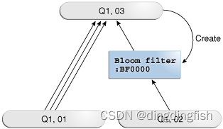

9.4.2 Partition-Wise Joins

Partition connection is an optimization , It joins two tables together （ One of them must be partitioned on the connection key ） Split into smaller connections .

Partition connection is one of the following ：

• Fully partitioned connection
  Two tables must be equally partitioned on their join keys , Or use reference partitions （ namely , Associated by reference constraints ）. A database divides a large connection into small connections between two partitions of two connection tables .
• Partial partition connection
  Only one table is partitioned on the join key . Another table may be partitioned , It may not be partitioned .

9.4.2.1 Purpose of Partition-Wise Joins

When the connection is executed in parallel , Partitioned connections reduce query response time by minimizing the amount of data exchanged between parallel execution servers .

This technology significantly reduces response time and improves CPU And memory usage . stay Oracle Real application clusters (Oracle RAC) Environment , Partitioned connections can also avoid or at least limit data traffic on the interconnect , This is the key to achieving good scalability for large-scale connection operations .

9.4.2.2 How Partition-Wise Joins Work

When the database serially connects two partitioned tables without using intelligent partitioned connection , A single server process performs a connection .

In the following illustration , The connection is not partitioned , Because the server process will table t1 Each partition of is connected to the table t2 Every section of .

It feels a bit like Cartesian product .

9.4.2.2.1 How a Full Partition-Wise Join Works

The database performs a fully intelligent partition connection in a serial or parallel manner .

The following figure shows a full partition connection executed in parallel . under these circumstances , Parallel granularity is a partition . Each parallel execution server joins the partition in pairs . for example , The first parallel execution server will t1 The first partition of is connected to t2 The first section of . Then the coordinator assembly results are executed in parallel .

Full partition connection can also connect partitions to child partitions , This is useful when tables use different partitioning methods . for example , Customers are partitioned by hash , But the sales are divided by range . If you are hashing sales Sub partition , Then the database can be in the customer's hash partition and sales Perform a complete partition connection between the hash sub partitions of .

In the execution plan , The existence of partition operation before connection indicates that there is a complete partition connection , This is shown in the following code snippet ：

|   8 |         PX PARTITION HASH ALL|
|*  9 |          HASH JOIN           |

9.4.2.2.2 How a Partial Partition-Wise Join Works

Unlike a full partition connection , Partial partition connections must be executed in parallel .

The following figure shows the partitioned t1 And unpartitioned t2 Partial partition connection between .

because t2 There is no division , A set of parallel execution servers must be started from as needed t2 Generate partition . then , A different set of parallel execution servers will t1 Partitions are connected to dynamically generated partitions . Parallel Execution Coordinator assembly results .

In the execution plan , operation PX SEND PARTITION (KEY) Indicates partial partition connection , As shown in the following code snippet ：

|  11 |            PX SEND PARTITION (KEY)    |

9.4.3 In-Memory Join Groups

Connection groups are user created objects , It lists two or more columns that can be meaningfully joined .

In some queries , Connection groups eliminate the performance overhead of understanding compression and hash values . Joining a group requires in memory column storage （IM Column store ）.