Simple dialogue system -- implement transformer by yourself

introduction

What we learned in the last article Transformer library , Just to understand Transformer, This passage PyTorch Achieve one Transformer, And complete the task of Chinese and English machinetranslation .

Package guide and initialization

import copy
import math
import matplotlib.pyplot as plt
import numpy as np
import os
import seaborn as sns
import time
import torch
import torch.nn as nn
import torch.nn.functional as F

from collections import Counter
from langconv import Converter
from nltk import word_tokenize
from torch.autograd import Variable

among nltk For the installation of, please refer to the article https://zhuanlan.zhihu.com/p/347931749
or

import nltk
nltk.set_proxy('http://proxy.example.com:3128', ('USERNAME', 'PASSWORD'))
nltk.download()

Initialization parameter settings ：

#  Initialization parameter settings 
PAD = 0                             # padding Index of placeholder 
UNK = 1                             #  Index of unlisted word identifiers 
BATCH_SIZE = 128                    #  Batch size 
EPOCHS = 20                         #  Number of training rounds 
LAYERS = 6                          # transformer in encoder、decoder The layer number 
H_NUM = 8                           #  The number of bulls' attention 
D_MODEL = 256                       #  Input 、 Output word vector dimension 
D_FF = 1024                         # feed forward Dimension of full connection layer 
DROPOUT = 0.1                       # dropout The proportion 
MAX_LENGTH = 60                     #  The maximum length of a statement 

TRAIN_FILE = 'nmt/en-cn/train.txt'  #  Training set 
DEV_FILE = "nmt/en-cn/dev.txt"      #  Verification set 
SAVE_FILE = 'save/model.pt'         #  Model save path 
DEVICE = torch.device("cuda" if torch.cuda.is_available() else "cpu")

Data preprocessing

The main thing to do is to load data 、 participle 、 Build vocabulary and batch partition . Generally speaking, Chinese sentences are written in word Cut for units , So there is no need to segment Chinese sentences .

The training data looks like this ：

Anyone can do that.	 Anyone can do .
How about another piece of cake?	 Would you like another piece of cake ？
She married him.	 She married him .
I don't like learning irregular verbs.	 I don't like learning irregular verbs .
It's a whole new ball game for me.	 This is a new ball game for me .
He's sleeping like a baby.	 He is asleep , Like a baby .
He can play both tennis and baseball.	 He can play tennis , I can play baseball again .
We should cancel the hike.	 We should cancel the hike .
He is good at dealing with children.	 He is good at dealing with children .

First, we populate the data by batch , Align the data length in the same batch .

def seq_padding(X, padding=PAD):
    """  By batch （batch） Fill in the data 、 Length alignment  """
    #  Calculate the length of each sample statement of the batch 
    lens = [len(x) for x in X]
    #  Get the maximum statement length in the batch sample 
    max_len = max(lens)
    #  Traverse the samples of this batch , If the statement length is less than the maximum length , Then use padding fill 
    return np.array([
        np.concatenate([x, [padding] * (max_len - len(x))]) if len(x) < max_len else x for x in X
    ])

The maximum length in different batches can be different .
As mentioned to see , The Chinese here is traditional , So we also need to do simple and complex conversion ：

def cht_to_chs(sent):
    sent = Converter("zh-hans").convert(sent)
    sent.encode("utf-8")
    return sent

Let's prepare the data ：

class PrepareData:
    def __init__(self, train_file, dev_file):
        #  Reading data 、 participle 
        self.train_en, self.train_cn = self.load_data(train_file)
        self.dev_en, self.dev_cn = self.load_data(dev_file)
        #  Building a vocabulary 
        self.en_word_dict, self.en_total_words, self.en_index_dict = \
            self.build_dict(self.train_en)
        self.cn_word_dict, self.cn_total_words, self.cn_index_dict = \
            self.build_dict(self.train_cn)
        #  Words are mapped to indexes 
        self.train_en, self.train_cn = self.word2id(self.train_en, self.train_cn, self.en_word_dict, self.cn_word_dict)
        self.dev_en, self.dev_cn = self.word2id(self.dev_en, self.dev_cn, self.en_word_dict, self.cn_word_dict)
        #  Divide the batch 、 fill 、 Mask 
        self.train_data = self.split_batch(self.train_en, self.train_cn, BATCH_SIZE)
        self.dev_data = self.split_batch(self.dev_en, self.dev_cn, BATCH_SIZE)

    def load_data(self, path):
        """  Read English 、 Chinese data   Segment each sample word and build a word list containing the start and end characters   In the form of ：en = [['BOS', 'i', 'love', 'you', 'EOS'], ['BOS', 'me', 'too', 'EOS'], ...] cn = [['BOS', ' I ', ' Love ', ' you ', 'EOS'], ['BOS', ' I ', ' also ', ' yes ', 'EOS'], ...] """
        en = []
        cn = []
        with open(path, mode="r", encoding="utf-8") as f:
            for line in f.readlines():
                sent_en, sent_cn = line.strip().split("\t")
                sent_en = sent_en.lower()
                sent_cn = cht_to_chs(sent_cn)
                sent_en = ["BOS"] + word_tokenize(sent_en) + ["EOS"]
                #  Chinese character segmentation 
                sent_cn = ["BOS"] + [char for char in sent_cn] + ["EOS"]
                en.append(sent_en)
                cn.append(sent_cn)
        return en, cn
    
    def build_dict(self, sentences, max_words=5e4):
        """  Construct the list data after word segmentation   Word construction - Index mapping （key For the word ,value by id value ） """
        #  Statistics of word frequency in the data set 
        word_count = Counter([word for sent in sentences for word in sent])
        #  Keep the former according to word frequency max_words Words to build a dictionary 
        #  add to UNK and PAD Two words 
        ls = word_count.most_common(int(max_words))
        total_words = len(ls) + 2
        word_dict = {
    w[0]: index + 2 for index, w in enumerate(ls)}
        word_dict['UNK'] = UNK
        word_dict['PAD'] = PAD
        #  structure id2word mapping 
        index_dict = {
    v: k for k, v in word_dict.items()}
        return word_dict, total_words, index_dict

    def word2id(self, en, cn, en_dict, cn_dict, sort=True):
        """  Will English 、 Turn the Chinese word list into the word index list  `sort=True` Means to sort by English sentence length , So that when filling by batch , The same batch of statements should be filled as little as possible  """
        length = len(en)
        #  Words are mapped to indexes 
        out_en_ids = [[en_dict.get(word, UNK) for word in sent] for sent in en]
        out_cn_ids = [[cn_dict.get(word, UNK) for word in sent] for sent in cn]
        #  Sort by statement length , Make the length within the batch as consistent as possible 
        def len_argsort(seq):
            """  Pass in a series of statement data ( Sort out the list of words ),  After sorting by statement length , Returns the index subscript of the original statements in the data after sorting  """
            return sorted(range(len(seq)), key=lambda x: len(seq[x]))
        #  In the same order 、 English sample sorting 
        if sort:
            #  Sort by English sentence length 
            sorted_index = len_argsort(out_en_ids)
            out_en_ids = [out_en_ids[idx] for idx in sorted_index]
            out_cn_ids = [out_cn_ids[idx] for idx in sorted_index]
        return out_en_ids, out_cn_ids

    def split_batch(self, en, cn, batch_size, shuffle=True):
        """  Divide the batch  `shuffle=True` It means random disorder of the sequence of each batch  """
        #  every other batch_size Take an index as a follow-up batch The starting index of 
        idx_list = np.arange(0, len(en), batch_size)
        #  The starting index is randomly scrambled 
        if shuffle:
            np.random.shuffle(idx_list)
        #  The statement index of all batches 
        batch_indexs = []
        for idx in idx_list:
            """  Form like [array([4, 5, 6, 7]), array([0, 1, 2, 3]), array([8, 9, 10, 11]), ...] """
            #  The batch with the largest initial index may be out of range , To qualify its index 
            batch_indexs.append(np.arange(idx, min(idx + batch_size, len(en))))
        #  Build a batch list 
        batches = []
        for batch_index in batch_indexs:
            #  Sample according to the sample index of the current batch 
            batch_en = [en[index] for index in batch_index]
            batch_cn = [cn[index] for index in batch_index]
            #  Fill all statements in the current batch 、 Align length 
            #  Dimension for ：batch_size *  Maximum length of statements in the current batch 
            batch_cn = seq_padding(batch_cn)
            batch_en = seq_padding(batch_en)
            #  Add the current batch to the batch list 
            # Batch Class is used to implement the attention mask 
            batches.append(Batch(batch_en, batch_cn))
        return batches

The data is ready , Now let's begin to understand Transformer Model .

Transformer Model overview

Transformer comparison LSTM The biggest advantage is that you can train in parallel , Greatly speed up computational efficiency . Understanding the order of language through location coding , Using self attention mechanism and full connection layer forward computing , There is no circular structure in the whole architecture .

Learn from it seq2seq,Transformer The model consists of encoder and decoder .

• Encoder (encoder)： Encoding natural language sequences into hidden layer representations
• decoder (decoder)： Mapping hidden layer representations to natural language sequences , So as to solve various tasks , Like emotional analysis 、 Named entity recognition and machine translation .

Let's look at the components in detail .

Word embedding layer

There are word embedding layers in both encoder and decoder , Used to input 、 Output ont-hot Vector mapping is word embedding vector . It can be initialized randomly for learning , You can also load pre trained word vectors .
Its implementation is relatively simple ：

class Embeddings(nn.Module):
    def __init__(self, d_model, vocab):
        super(Embeddings, self).__init__()
        # Embedding layer 
        self.embed = nn.Embedding(vocab, d_model)
        # Embedding dimension 
        self.d_model = d_model

    def forward(self, x):
        #  return x The word of the vector （ It needs to be multiplied by math.sqrt(d_model)）
        return self.embed(x) * math.sqrt(self.d_model)

Location code

because Transformer The input of is in parallel , Missing word location information . Therefore, it is necessary to add a location coding layer containing word location information .

Location code （positional encoding）： The position coding vector has the same dimension as the word vector ,$\text{max\_seq\_len}\times \text{embedding\_dim}$.

Transformer In the original text, the positive is used 、 The linear transformation of cosine function encodes the word position ：

$$\begin{gathered} {\text{PE}}_{pos,2i}=\sin \left(\frac{pos}{10000^{2i/d_{\text{model}}}}\right) \\ {\text{PE}}_{(pos,2i+1)}=\cos \left(\frac{pos}{10000^{2i/d_{\text{model}}}}\right)\text{\hspace{1em}(1)} \end{gathered}$$

In order to use sequence order information , The author proposes to use sine and cosine functions of different frequencies to represent position coding . The importance of sequence information is self-evident . For example, the following two sentences ：

 I love you! 
 You love me 

The author uses word embedding vector position coding to get the input vector , Here is a brief explanation of why the author chooses sine and cosine functions .

Suppose we set the location code ourselves , A simple way is to add an index to the word embedding vector .

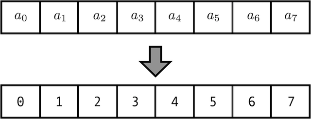
hypothesis $a$ The representation is embedded in the vector . There is a big problem with this method , That is, the longer the sentence , The larger the serial number of the following words , And the index value is too large , May mask the embedded vector “ glorious ”.

You said the serial number is too big , So it's not big for me to divide each serial number by the length of the sentence . That sounds good , But this introduces another problem , Because the length of the sentence is different , Leading to the same value may mean different things , This makes our model very confused . such as $0.8$ In the sentence, the length is $5$ In the sentence of $4$ Word , But when the sentence is long $20$ In the sentence of $16$ Word .

Because the length of the sentence above is 8,$2^3=8$, Why not use binary to represent sequence information ？ As shown in the figure above . From the top down , such as 4 Corresponding “100”,5 Corresponding “101”.

Here we use 3 Bit representation is enough , Generally, we can set it to $d_{model}$.

Is this a good method ？

1. We are still not fully normalized . We want the location code to conform to a certain distribution . It's best to make positive and negative numbers evenly distributed , This is a good implementation , You can do this through a function $f(x)=2x-1$, take [0,1] -> [-1,1]
2. Our binary vectors come from discrete functions , Instead of discretization of continuous functions .

Our location code should meet the following requirements ：

1. For each time step ( The word position in the sentence ), It can output unique codes
2. The distance between any two time steps should be a constant , It doesn't change with the length of the sentence
3. Our model should be easily generalized to longer sentences , Its value should be bounded
4. The location code must be deterministic

The coding method proposed by the author is a simple and talented Technology , All the above requirements are met . First , It's not a scalar , It's a that contains location specific information $d$ Dimension vector . secondly , The code is not integrated into the model . contrary , This vector is used to set information for each word about its position in the sentence . In other words , Enhance the input of the model by injecting the order of words .

Make $t$ For a position in the input sequence ,$\overrightarrow{p_t}$ Is the location code of the location ,$d$ It's a vector dimension .$f$ Is a function of generating a position coding vector by the following formula ：
$${\overrightarrow{p_t}}^{(i)}=f(t{)}^{(i)}:=\{\begin{array}{ll}\sin ({\omega }_k\cdot t),& \text{if}i=2k\\ \cos ({\omega }_k\cdot t),& \text{if}i=2k+1\end{array}$$
among
$${\omega }_k=\frac{1}{10000^{2k/d}}$$
From this equation, we can see , The frequency decreases with the vector dimension ( from $\frac{1}{2\pi }$ Reduced to $\frac{1}{10000\cdot 2\pi }$). Therefore, the wavelength forms a from $2\pi$ To $10000\cdot 2\pi$ A series of equal proportions .

We can also imagine location coding $\overrightarrow{p_t}$ Is a sine and cosine vector containing each frequency , among $d$ Can be $2$ to be divisible by .
$$\overrightarrow{p_t}={\left[\begin{array}{c}\sin ({\omega }_1\cdot t)\\ \cos ({\omega }_1\cdot t)\\ \\ \sin ({\omega }_2\cdot t)\\ \cos ({\omega }_2\cdot t)\\ \\ ⋮\\ \\ \sin ({\omega }_{d/2}\cdot t)\\ \cos ({\omega }_{d/2}\cdot t)\end{array}\right]}_{d\times 1}$$
Why can the combination of sine and cosine represent order . Suppose we use binary to represent numbers .
$$\begin{array}{rlr}0:\text{0}\text{0}\text{0}\text{0}& & 8:\text{1}\text{0}\text{0}\text{0}\\ 1:\text{0}\text{0}\text{0}\text{1}& & 9:\text{1}\text{0}\text{0}\text{1}\\ 2:\text{0}\text{0}\text{1}\text{0}& & 10:\text{1}\text{0}\text{1}\text{0}\\ 3:\text{0}\text{0}\text{1}\text{1}& & 11:\text{1}\text{0}\text{1}\text{1}\\ 4:\text{0}\text{1}\text{0}\text{0}& & 12:\text{1}\text{1}\text{0}\text{0}\\ 5:\text{0}\text{1}\text{0}\text{1}& & 13:\text{1}\text{1}\text{0}\text{1}\\ 6:\text{0}\text{1}\text{1}\text{0}& & 14:\text{1}\text{1}\text{1}\text{0}\\ 7:\text{0}\text{1}\text{1}\text{1}& & 15:\text{1}\text{1}\text{1}\text{1}\end{array}$$

You can see , With the increase of decimal numbers , The rate of change of each bit is different , The lower the level, the faster the change , Red bit $0$ and $1$, Every number changes once ;

And the Yellow bit , Every time $8$ A number changes once .

But binary values $0,1$ Is discrete , Wasted infinite floating-point numbers between them . So we use their continuous floating versions - Sine function .

Besides , By reducing their frequency , We can change from red to yellow , This realizes the transformation from low to high . As shown in the figure below ：

Let's add the calculation of wavelength and frequency ：

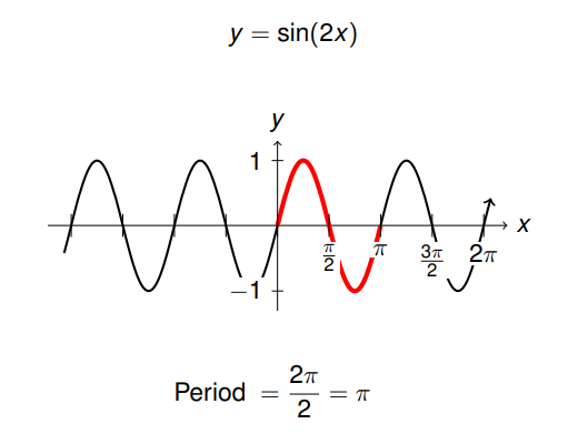
For sinusoidal functions , wavelength ( cycle ) The calculation is shown in the figure above . arbitrarily $\sin (Bx)$ The wavelength is $\frac{2\pi }{B}$, The frequency is $\frac{B}{2\pi }$.

Last , By setting the dimension of position coding to be consistent with that of word embedding vector , You can add position coding to the word vector .

It is mentioned in the original

For any fixed offset $k$,$P{E}_{pos+k}$ Must be able to express as $P{E}_{pos}$ A linear function of .

The top of the figure above is a length of 200、 Dimension for 150 The transposed position matrix of the sequence $PE$, At the bottom of the figure above is the $p$ The... In the position vector of $i$ Sine cosine function image of component positions , come from Hands-on Machine Learning with Scikit Learn, Keras, TensorFlow: Concepts, Tools and Techniques to Build Intelligent Systems 2nd Edition

For each frequency ${\omega }_k$ The corresponding positive - Cosine pair , There is a linear transformation $M\in {\mathbb{R}}^{2\times 2}$：
$$M.\left[\begin{array}{c}\sin ({\omega }_k\cdot t)\\ \cos ({\omega }_k\cdot t)\end{array}\right]=\left[\begin{array}{c}\sin ({\omega }_k\cdot (t+\varphi ))\\ \cos ({\omega }_k\cdot (t+\varphi ))\end{array}\right]$$

prove ：

hypothesis $M$ It's a $2\times 2$ Matrix , We want to find the elements $u_1,v_1,u_2,v_2$ Satisfy ：
$$\left[\begin{array}{cc}{u}_1& v_1\\ u_2& v_2\end{array}\right]\cdot \left[\begin{array}{c}\sin ({\omega }_k\cdot t)\\ \cos ({\omega }_k\cdot t)\end{array}\right]=\left[\begin{array}{c}\sin ({\omega }_k\cdot (t+\varphi ))\\ \cos ({\omega }_k\cdot (t+\varphi ))\end{array}\right]$$
Using the sine formula and cosine formula of the sum of two angles of trigonometric function , obtain ：

$$\left[\begin{array}{cc}{u}_1& v_1\\ u_2& v_2\end{array}\right]\cdot \left[\begin{array}{c}\sin ({\omega }_k\cdot t)\\ \cos ({\omega }_k\cdot t)\end{array}\right]=\left[\begin{array}{c}\sin ({\omega }_k\cdot t)\cos ({\omega }_k\cdot \varphi )+\cos ({\omega }_k\cdot t)\sin ({\omega }_k\cdot \varphi )\\ \cos ({\omega }_k\cdot t)\cos ({\omega }_k\cdot \varphi )-\sin ({\omega }_k\cdot t)\sin ({\omega }_k\cdot \varphi )\end{array}\right]$$
Get the following two equations ：
$$\begin{array}{rl}{u}_1\sin ({\omega }_k\cdot t)+v_1\cos ({\omega }_k\cdot t)=& \cos ({\omega }_k\cdot \varphi )\sin ({\omega }_k\cdot t)+\sin ({\omega }_k\cdot \varphi )\cos ({\omega }_k\cdot t)\\ u_2\sin ({\omega }_k\cdot t)+v_2\cos ({\omega }_k\cdot t)=& -\sin ({\omega }_k\cdot \varphi )\sin ({\omega }_k\cdot t)+\cos ({\omega }_k\cdot \varphi )\cos ({\omega }_k\cdot t)\end{array}$$
Corresponding , Available ：
$$\begin{array}{rl}{u}_1=\cos ({\omega }_k.\varphi )& v_1=\sin ({\omega }_k.\varphi )\\ u_2=-\sin ({\omega }_k.\varphi )& v_2=\cos ({\omega }_k.\varphi )\end{array}$$
therefore , You get the final matrix $M$ by ：
$$M_{\varphi ,k}=\left[\begin{array}{cc}\cos ({\omega }_k\cdot \varphi )& \sin ({\omega }_k\cdot \varphi )\\ -\sin ({\omega }_k\cdot \varphi )& \cos ({\omega }_k\cdot \varphi )\end{array}\right]$$
And you can see that , The final conversion and $t$ irrelevant .

Similarly , We can find other positive - Cosine right $M$, Finally allow us to express $\overrightarrow{p_{t+\varphi }}$ For one $\overrightarrow{p_t}$ For any fixed offset $\varphi$ The linear function of . This attribute , Make it easy for the model to learn the relative position information .

This explains why we choose alternating sine and cosine functions , This cannot be achieved only by sine or cosine functions .

We implement location coding as follows ：

class PositionalEncoding(nn.Module):
    def __init__(self, d_model, dropout, max_len=5000):
        super(PositionalEncoding, self).__init__()
        self.dropout = nn.Dropout(p=dropout)
        #  Location coding matrix , dimension [max_len, embedding_dim]
        pe = torch.zeros(max_len, d_model, device=DEVICE)
        #  Word position 
        position = torch.arange(0.0, max_len, device=DEVICE)
        position.unsqueeze_(1)
        #  Use exp and log Implement power operation 
        div_term = torch.exp(torch.arange(0.0, d_model, 2, device=DEVICE) * (- math.log(1e4) / d_model))
        div_term.unsqueeze_(0)
        #  Calculate the texture value of the word position along the word vector dimension 
        pe[:, 0 : : 2] = torch.sin(torch.mm(position, div_term))
        pe[:, 1 : : 2] = torch.cos(torch.mm(position, div_term))
        #  Add batch dimension ,[1, max_len, embedding_dim]
        pe.unsqueeze_(0)
        #  Register the location code matrix as buffer( No training ), Because it is an absolute location code 
        self.register_buffer('pe', pe)

    def forward(self, x):
        #  Add all word vectors and position codes of statements in a batch 
        #  Be careful , Position coding does not participate in training , So set requires_grad=False
        x += Variable(self.pe[:, : x.size(1), :], requires_grad=False)
        return self.dropout(x)

Encoder

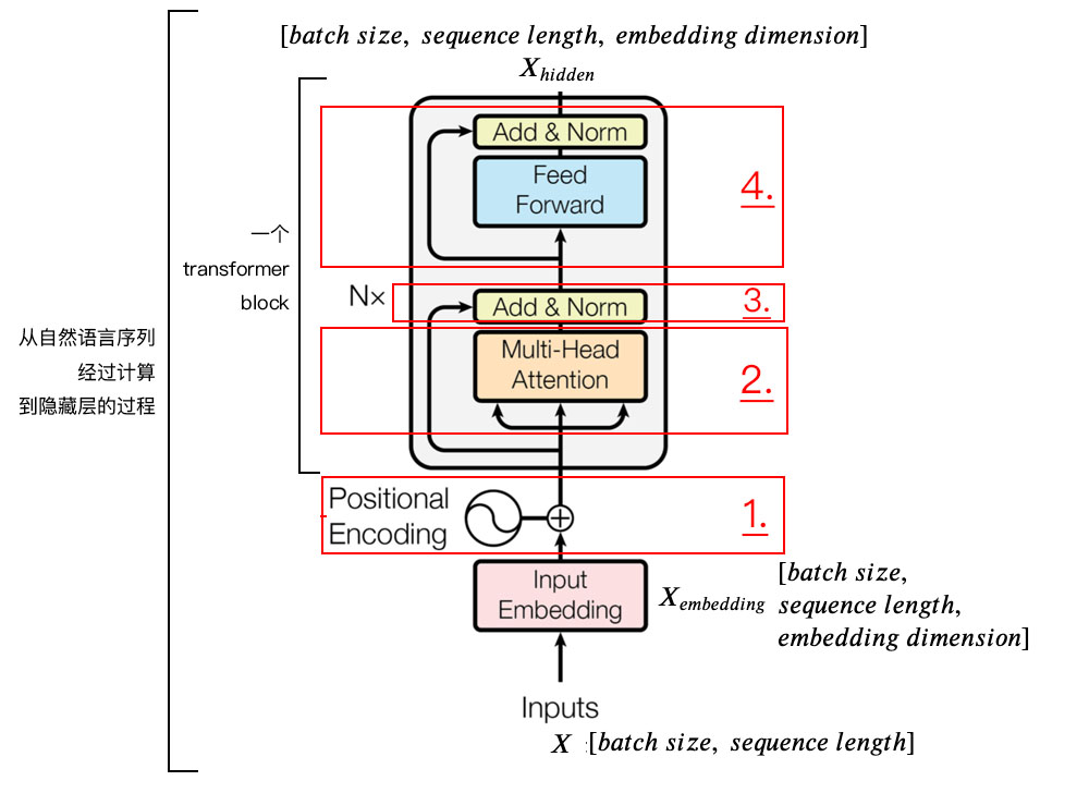
The encoder is embedded by the input + Location code +Transformer block (block) form .
Used to transform natural language sequences into hidden state representations , Can complete some mainstream NLP Mission , Such as emotional classification 、 Semantic relationship analysis and named entity recognition .
Where input $X$ yes batch size A length of sequence length The only hot code ; Through the input embedded layer , Added embedded dimension ; And then pass by Transformer Block for more complex transformations .

stay Transformer There is a lot of attention in the block 、 Residual connection 、 Layer normalization and feedforward neural network . Let's take a look at them separately .

Self attention

We now have word vector sentences and position embedding , Suppose we have some sentences $X$, Its shape is [batch_size,sequence_length], First, we find the corresponding embedding in the word vector , Then add it to the positional embedded element , Get the final embedded $X_{embedding}$ Shape is ：[batch_size,sequence_length,embedding_dimension].

As shown in the figure above ,$X_{embedding}$ The calculation formula of is ：
$$X_{embedding}=EmbeddingLookup(X)+PositioinalEncoding(X)\text{\hspace{1em}(2)}$$

next , In order to learn the expression of multiple meanings , Yes $X_{embedding}$ Do linear mapping , Multiply by three weights $W_Q,W_K,W_V\in {\mathbb{R}}^{embed\_dim\times embed\_dim}$：
$$\begin{array}{rl}Q& =Linear(X_{embedding})=X_{embedding}{W}_Q\\ K& =Linear(X_{embedding})=X_{embedding}{W}_K\\ V& =Linear(X_{embedding})=X_{embedding}{W}_V\end{array}\text{\hspace{1em}(3)}$$

Then get ready for long attention , Why is it a bull ？
Because we need to use attention mechanism to extract multiple semantics , We first define a super parameter $h$, namely head The number of , Dimension embedded here (embedding dimension) Must be divisible by $h$, Because we want to divide the embedded dimension into $h$ Share .

At the end of the figure above, we split the embedded dimension into $h$ Share , After split $Q,K,V$ The dimensions are [batch_size,sequence_length,h,embedding_dimension / h], Then we put $Q,K,V$ Medium sequence_length,h A bit of transposing , In order to facilitate the subsequent calculation . The transposed $Q,K,V$ The dimensions are [batch_size,h,sequence_length,embedding_dimension / h].

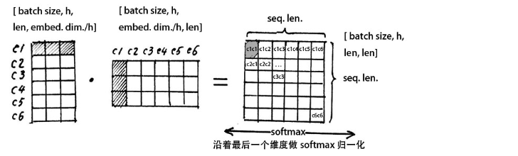
Above picture , Let's take out a group heads To explain the meaning of long attention . Let's take out a group heads, That is, a group of split $Q,K,V$, Their dimensions are [sequence_length,embedding_dimension / h], Let's calculate first $Q$ And $K$ The transposed dot product of , Note their dimensions in the figure above .
The more similar the two vectors are , The larger their dot product .
Here we first use the word which stands for the first word $c1$ Line with $c1$ Column multiplication , I get a number , In the attention matrix ( The matrix on the far right of the figure above ) Of the $1$ Xing di $1$ Column $c1c1$, Here stands for the first word and your attention score , And then we can find out in turn $c1c2,c1c3,\cdots$.

The first line of the attention matrix represents which of the six words the first word is related to .
$$\text{Attention}(Q,K,V)=\text{softmax}(\frac{Q{K}^T}{\sqrt{d_k}})V\text{\hspace{1em}(4)}$$
In the above formula is the self attention mechanism , Let's ask first $Q{K}^T$, That is to find the attention matrix , Then use the attention matrix to $V$ weighting ,$\sqrt{d_k}$ In order to change the attention matrix into a standard normal distribution , bring softmax The result after normalization is more stable .

Now we have the attention matrix , And use softmax normalization , Make the sum of attention weights of each word and all other words equal to $1$, The function of attention matrix is a probability distribution of attention weight , We're going to use the weight of the attention matrix to give $V$ Weighted , In the figure above, we take a row from the attention matrix ( And for $1$), Then point by point $V$ The column of .
matrix $V$ Each line of represents the mathematical expression of each word vector , Our above operation is the weighted linear combination of these mathematical expressions of attention weight , So that each word vector contains the information of all word vectors in the current sentence .

Note that after dot product operation ,$V$ There is no change in the dimension of , still [batch_size,h,sequence_length,embedding_dimension / h].

Here's a simple example ：

$\sqrt{d_k}$ normalization

hypothesis $\mathbf{q}$、$\mathbf{k}$ Is the mean 0、 variance 1 Of independent random variables , Its dot accumulates attention $\mathbf{q}\cdot \mathbf{k}={\sum }_{i=1}^{d_k}{\mathbf{q}}_i{\mathbf{k}}_i$ The mean and variance of are 0、$d_k$. adopt $\sqrt{d_k}$ The zoom , send softmax The results are more stable （ Prevent words - The dot product attention difference between words is too big ）, It is convenient for gradient balance in back propagation .

Now let's realize the multi head attention , First, implement the clone help function ：

def clones(module, N):
    """  Clone base unit , Parameters are not shared between cloned cells  """
    return nn.ModuleList([
        copy.deepcopy(module) for _ in range(N)
    ])

Then we implement the zoom attention calculation function ：

def attention(query, key, value, mask=None, dropout=None):
    """ Scaled Dot-Product Attention(  The formula (4) ) """
    # q、k、v The length of the vector is d_k
    d_k = query.size(-1)
    #  Matrix multiplication implementation q、k Dot product attention ,sqrt(d_k) normalization 
    scores = torch.matmul(query, key.transpose(-2, -1)) / math.sqrt(d_k)
    #  Attention mask mechanism 
    if mask is not None:
        scores = scores.masked_fill(mask==0, -1e9)
    #  Attention matrix softmax normalization 
    p_attn = F.softmax(scores, dim=-1)
    # dropout
    if dropout is not None:
        p_attn = dropout(p_attn)
    #  Attention is right v weighting 
    return torch.matmul(p_attn, value), p_attn

Finally, we will implement the multi head attention layer ：

class MultiHeadedAttention(nn.Module):
    """ Multi-Head Attention（ Encoder No 2 part ） """
    def __init__(self, h, d_model, dropout=0.1):
        super(MultiHeadedAttention, self).__init__()
        """ `h`： The number of attention heads  `d_model`： Word vector dimension  """
        #  Make sure you divide 
        assert d_model % h == 0
        # q、k、v Vector dimension 
        self.d_k = d_model // h
        #  The number of heads 
        self.h = h
        # WQ、WK、WV Matrix and multi head attention splicing transformation matrix WO
        self.linears = clones(nn.Linear(d_model, d_model), 4)
        self.attn = None
        self.dropout = nn.Dropout(p=dropout)

    def forward(self, query, key, value, mask=None):
        if mask is not None:
            mask = mask.unsqueeze(1)
        #  Batch size 
        nbatches = query.size(0)
        # WQ、WK、WV Linear transformation of word vectors respectively , And split the results into h block 
        query, key, value = [
            l(x).view(nbatches, -1, self.h, self.d_k).transpose(1, 2)
            for l, x in zip(self.linears, (query, key, value))
        ]
        #  Attention weighting 
        x, self.attn = attention(query, key, value, mask=mask, dropout=self.dropout)
        #  Multi head attention weighted splicing 
        x = x.transpose(1, 2).contiguous().view(nbatches, -1, self.h * self.d_k)
        #  Linear transformation of multi head attention weighted stitching results 
        return self.linears[-1](x)

The above code implements the multi head attention shown in the figure above , Attention there is actually 4 It's a linear transformation , Corresponding to the above self.linears = clones(nn.Linear(d_model, d_model), 4), Namely $Q,K,V$ And the one following the top splicing Linear layer .

Layer normalization

Layer normalization normalizes each dimension of each input . Suppose there is $H$ Dimensions ,$x=(x_1,x_2,\cdots ,x_H)$, Layer normalization first calculates this $H$ Mean and variance of dimensions , Then normalize to get $N(x)$, Then do a zoom , Similar to batch normalization .

$$\mu =\frac{1}{H}\sum _{i=1}^H{x}_i,\sigma =\sqrt{\frac{1}{H}\sum _{i=1}^H(x_i-\mu {)}^2},N(x)=\frac{x-\mu }{\sigma },h=\alpha \odot N(x)+\beta \text{\hspace{1em}(5)}$$
among ,$\odot$ Express Hadamard product , That is, the corresponding elements of two vectors are multiplied ;$h$ Namely LN Layer output ;$\mu$ and $\sigma$ Is to input the mean and variance of each dimension ;$\alpha$ and $\beta$ Are two learnable parameters ; and $h$ The dimensions of are the same .

class LayerNorm(nn.Module):
    def __init__(self, features, eps=1e-6):
        super(LayerNorm, self).__init__()
        # α、β They are initialized to 1、0
        self.a_2 = nn.Parameter(torch.ones(features))
        self.b_2 = nn.Parameter(torch.zeros(features))
        #  Smooth items 
        self.eps = eps

    def forward(self, x):
        #  Calculate the mean and variance along the word vector 
        mean = x.mean(dim=-1, keepdim=True)
        std = x.std(dim=-1, keepdim=True)
        #  Calculate the mean and variance along the word vector and sentence sequence 
        # mean = x.mean(dim=[-2, -1], keepdim=True)
        # std = x.std(dim=[-2, -1], keepdim=True)
        #  normalization 
        x = (x - mean) / torch.sqrt(std ** 2 + self.eps)
        return self.a_2 * x + self.b_2

Residual connection

Suppose a layer in the network inputs $x$ The output of the system is $F(x)$, Whatever the activation function is , Passing through the deep network may lead to the disappearance of the gradient . Add residual connection , Equivalent to a layer of input $x$ The output of the system is $F(x)+x$. The worst case scenario is equivalent to not going through $F(x)$ This floor , Input directly to the high level , In this way, the high-level performance can be at least as good as the low-level performance .

here $\text{SubLayer}$ That's what it says $F$. During training , The gradient is directly back propagated to the front layer through a shortcut

$$\mathbf{x}+\text{SubLayer}(\mathbf{x})\text{\hspace{1em}(6)}$$

among ,$\text{SubLayer}$ Express Add & Norm Front layer module , Such as Multi-Head Attention、Feed Forward.

class SublayerConnection(nn.Module):
    """  Encapsulates layer normalization and residual linking , In the middle of the sublayer It is a multi head attention or feedforward network  """
    def __init__(self, size, dropout):
        super(SublayerConnection, self).__init__()
        self.norm = LayerNorm(size)
        self.dropout = nn.Dropout(dropout)

    def forward(self, x, sublayer):
        #  Layer normalization 
        x_ = self.norm(x)
        #  The real sublayer ( Multi head attention or feedforward network )
        x_ = sublayer(x_)
        #  We have to go through Dropout
        x_ = self.dropout(x_) 
        #  Residual connection 
        return x + x_

Feedforward networks

Feedforward networks （Feed Forward） It is a two-level linear mapping and activation function .

class PositionwiseFeedForward(nn.Module):
    def __init__(self, d_model, d_ff, dropout=0.1):
        super(PositionwiseFeedForward, self).__init__()
        self.w_1 = nn.Linear(d_model, d_ff) #  linear transformation 
        self.w_2 = nn.Linear(d_ff, d_model) #  linear transformation 
        self.dropout = nn.Dropout(dropout)

    def forward(self, x):
        x = self.w_1(x)
        x = F.relu(x)
        x = self.dropout(x)
        x = self.w_2(x)
        return x

Overall encoder architecture

Transformer The basic unit of the encoder consists of two sublayers ： The first sublayer implements multiple heads Self attention （self-attention Mechanism （Multi-Head Attention）; The second sublayer implements a fully connected feedforward network . The calculation process is as follows ：

1. Word vector and position coding

$$X=\text{EmbeddingLookup}(X)+\text{PositionalEncoding}\text{\hspace{1em}(7)}$$
obtain
$$X\in {\mathbb{R}}^{\text{batch\_size}\times \text{seq\_len}\times \text{embedding\_dim}}$$

2. Self attention mechanism

$$Q=\text{Linear}(X)=X{W}_Q$$

$$K=\text{Linear}(X)=X{W}_K\text{\hspace{1em}(8)}$$

$$V=\text{Linear}(X)=X{W}_V$$

$$X_{\text{attention}}=\text{SelfAttention}(Q,K,V)\text{\hspace{1em}(9)}$$

3. Layer normalization 、 Residual connection

$$X_{\text{attention}}=\text{LayerNorm}(X_{\text{attention}})\text{\hspace{1em}(10)}$$

$$X_{\text{attention}}=X+X_{\text{attention}}\text{\hspace{1em}(11)}$$

4. Feedforward networks

$$X_{\text{hidden}}=\text{Linear}(\text{Activate}(\text{Linear}(X_{\text{attention}})))\text{\hspace{1em}(12)}$$

5. Layer normalization 、 Residual connection

$$X_{\text{hidden}}=\text{LayerNorm}(X_{\text{hidden}})\text{\hspace{1em}(13)}$$

$$X_{\text{hidden}}=X_{\text{attention}}+X_{\text{hidden}}\text{\hspace{1em}(14)}$$
among
$$X_{\text{hidden}}\in {\mathbb{R}}^{\text{batch\_size}\times \text{seq\_len}\times \text{embedding\_dim}}$$

Transformer Encoder by $N=6$ It consists of three encoder basic units .

Then build on the above , Let's implement the encoder layer ：

class EncoderLayer(nn.Module):
    def __init__(self, size, self_attn, feed_forward, dropout):
        super(EncoderLayer, self).__init__()
        self.self_attn = self_attn #  Long attention 
        self.feed_forward = feed_forward #  Feedforward networks 
        # SublayerConnection Functional connection multi and ffn
        self.sublayer = clones(SublayerConnection(size, dropout), 2)
        # d_model
        self.size = size

    def forward(self, x, mask):
        #  take embedding Layer for multi head attention 
        x = self.sublayer[0](x, lambda x: self.self_attn(x, x, x, mask)) #  First, the attention of the Bulls 
        # attn The result of is directly input as the next layer 
        return self.sublayer[1](x, self.feed_forward) #  Then the feedforward network 

And the encoder is $N$ Superposition of encoder layers ：

class Encoder(nn.Module):
    def __init__(self, layer, N):
        """ layer = EncoderLayer """
        super(Encoder, self).__init__()
        #  Copy N Encoder basic unit 
        self.layers = clones(layer, N)
        #  Layer normalization 
        self.norm = LayerNorm(layer.size)
        
    def forward(self, x, mask):
        """  Cycle encoder basic unit N Time  """
        for layer in self.layers:
            x = layer(x, mask) #  superposition N Time 
        return self.norm(x) #  Finally, through layer normalization 

The encoder is understood , Let's look at the decoder .

decoder

The decoder is also composed of $N$ Layer decoder basic units are stacked , Different from the basic unit of the encoder ： The decoder is at the multiple ends of the encoder basic unit Self attention Between the mechanism and the feedforward network Context attention （context-attention Mechanism （Multi-Head Attention） layer , The output of the self attention mechanism of the basic unit of the decoder is used as $q$ Query the output of the encoder , So that when decoding , The decoder obtains all the outputs of the encoder , The mechanism of contextual attention $K$ and $V$ The output from the encoder ,$Q$ Output from the decoder at the previous moment .

You can see from the above picture that , Decoder yes 3 Sublayer (SubLayer).

Input of decoder basic unit 、 Output ：

• Input ： Output of encoder 、 The output of the decoder at the previous moment

• Output ： Corresponding to the probability distribution of the output word at the current time

Besides , The output of the decoder （ The output of the last decoder basic unit ） It requires a linear transformation and softmax The function map predicts the probability distribution of the word at the next moment .

decoder The decoding process ： Given encoder output （ The encoder inputs the word vector of all words in the statement ） And the decoder output at the previous moment （ word ）, Predict the probability distribution of words at the current time .

Be careful ： During training , Ed 、 The decoder can calculate in parallel （ The words of the previous moment are known in the training corpus ）; In the process of reasoning , Encoder can calculate in parallel , The decoder needs to be like RNN Predict the output words in turn .

Let's take a look at the implementation of the decoder layer ：

class DecoderLayer(nn.Module):
    def __init__(self, size, self_attn, src_attn, feed_forward, dropout):
        super(DecoderLayer, self).__init__()
        self.size = size
        #  Self attention mechanism 
        self.self_attn = self_attn
        #  Contextual attention mechanism 
        self.src_attn = src_attn
        #  Feedforward networks 
        self.feed_forward = feed_forward
        self.sublayer = clones(SublayerConnection(size, dropout), 3) #  The decoder has three sublayers 

    def forward(self, x, memory, src_mask, tgt_mask):
        # memory Hide representation for encoder output 
        m = memory
        #  Self attention mechanism ,q、k、v Both come from the decoder implicit representation  ( Sublayer 1 )
        x = self.sublayer[0](x, lambda x: self.self_attn(x, x, x, tgt_mask))
        #  Contextual attention mechanism ：q Implicitly represent for from decoder , and k、v Implicitly represent... For the encoder  ( Sublayer 2 )
        x = self.sublayer[1](x, lambda x: self.src_attn(x, m, m, src_mask))
        #  Next is the feedforward network ( Sublayer 3 )
        return self.sublayer[2](x, self.feed_forward)

Implementation of decoder , It is mainly cloning $N$ Two decoder layers , The final output is normalized by the layer ：

class Decoder(nn.Module):
    def __init__(self, layer, N):
        super(Decoder, self).__init__()
        self.layers = clones(layer, N)
        self.norm = LayerNorm(layer.size)
        
    def forward(self, x, memory, src_mask, tgt_mask):
        """  Loop decoder basic unit N Time  """
        for layer in self.layers:
            x = layer(x, memory, src_mask, tgt_mask)
        return self.norm(x)

The top part of the decoder acts as a generator (generator), By the linear layer +Softmax layers ：

class Generator(nn.Module):
    """  The output of the decoder is linearly transformed and softmax The function map predicts the probability distribution of the word at the next moment  """
    def __init__(self, d_model, vocab):
        super(Generator, self).__init__()
        # decode After the results of the , First enter a fully connected layer into a dictionary sized vector 
        self.proj = nn.Linear(d_model, vocab)

    def forward(self, x):
        #  And then we can move on log_softmax operation ( stay softmax As a result, do it again log operation )
        return F.log_softmax(self.proj(x), dim=-1)

Basically, the introduction is almost complete , There is one more detail —— Attention mask .

Attention mask

Attention mask plays different roles in encoder and decoder .

Encoder attention mask

We know , Natural language processing , Text statements are usually of different lengths in batch data , Therefore, it is necessary to fill in the phrase sentences , The filled characters do not need to participate in attention calculation .

therefore , The destination of the encoder attention mask ： Make the filled part of the phrase sentence in the batch not participate in the attention calculation .

Model training is usually carried out in batches , The length of statements in the same batch may be different , Therefore, it is necessary to modify the phrasal sentence according to the maximum length of the sentence 0 Fill to make up the length . Statement fill part is invalid information , Should not participate in forward communication , consider softmax Function properties ,

$$\text{softmax}(\mathbf{z}{)}_i=\frac{\exp (z_i)}{{\sum }_{j=1}^K\exp (z_j)}\text{\hspace{1em}(15)}$$

When $z_i$ When filling , May make $z_i=-\infty$（ Usually take a large negative number ） Make it invalid , namely

$$z_{\text{pad}}=-\infty \Rightarrow \exp (z_{\text{pad}})=0$$

Here we just need to set a large enough negative number , Encoder attention mask generates pseudo code ：

# True Indicates valid ;False Invalid representation （ Fill bit ）
mask = src != pad #  Here is matrix operation ,mask In Chinese, it means true Of is an unfilled character , by false Is filled with characters 
#  Set the invalid position to negative infinity 
scores = scores.masked_fill(~mask, -1e9) # ~mask, Take the opposite , Will be for false The padding character of is set to -1e9

Next, let's look at the decoder attention mask .

Decoder attention mask

The decoder attention mask is slightly more complex than the encoder , It is not only necessary to shield the filling part , It is also necessary to mask the current and subsequent sequences （subsequent_mask）, To prevent cheating .
That is, when the decoder predicts the word at the current time , Unable to know the current and subsequent word contents , Therefore, the attention mask needs to set all the attention scores after the current time to $-\infty$, And then calculate $softmax$, Prevent data leakage .

subsequent_mask Is a lower triangular matrix , The upper right position of the main diagonal is all False.

Let's take a look at how this shielding is done .

def subsequent_mask(size):
    '''  Add masking for the position of subsequent output sequences  :param size:  Output sequence length  '''
    attn_shape = (1, size, size)
    #  Move the main diagonal up one position , The elements below the main diagonal are all 0
    mask = np.triu(np.ones(attn_shape), k=1).astype('uint8')
    return torch.from_numpy(mask) == 0

np.triu do ？

np.triu(a, k) Is to take the matrix a Upper triangle data of , The slash position of the trigonometric data is determined by k decision , And below the slash are 0.

import numpy as np
a = np.arange(1,17).reshape(4,-1)
print(a)

[[ 1  2  3  4]
 [ 5  6  7  8]
 [ 9 10 11 12]
 [13 14 15 16]]

When np.triu(a, k = 0) when , Get the upper triangle data including the main diagonal .

print(np.triu(a, k = 0))

[[ 1  2  3  4]
 [ 0  6  7  8]
 [ 0  0 11 12]
 [ 0  0  0 16]]

When np.triu(a, k = 1) when , Move the main diagonal up one position .

print(np.triu(a, k = 1))

[[ 0  2  3  4]
 [ 0  0  7  8]
 [ 0  0  0 12]
 [ 0  0  0  0]]

When np.triu(a, k = -1) when , Move the main diagonal down one position .

print(np.triu(a, k = -1))

[[ 1  2  3  4]
 [ 5  6  7  8]
 [ 0 10 11 12]
 [ 0  0 15 16]]

attention mask Each... Is shown below tgt( The goal is ) word ( That's ok ) Locations allowed to view ( Column ). In the process of training , Words after the current word will be blocked .

plt.figure(figsize=(5,5))
plt.imshow(subsequent_mask(20)[0])

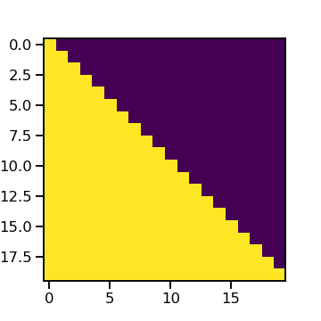
For example 0 That's ok , You can only see 1 Column , The first 1 Line can only see 2 Column . The yellow area represents the visible Columns .

At the end of this section , We can implement the batch class ,

class Batch:
    """  Batch type  1.  Input sequence （ Source ） 2.  Output sequence （ The goal is ） 3.  Construct mask  """
    def __init__(self, src, trg=None, pad=PAD):
        ''' :param src:  Source data  [batch_size, input_len] :param trg:  Target data  [batch_size, input_len] '''
        #  Enter 、 Output words id The data represented is normalized to integer type 
        src = torch.from_numpy(src).to(DEVICE).long()
        trg = torch.from_numpy(trg).to(DEVICE).long()
        self.src = src
        #  Judge the non empty part of the current input statement ,bool Sequence 
        #  And in seq length Add one dimension to the front , The formation dimension is  1×seq length  Matrix 
        self.src_mask = (src != pad).unsqueeze(-2)
        #  If the output destination is not empty , You need to mask the target statement used by the decoder 
        if trg is not None:
            #  The target input part used by the decoder 
            self.trg = trg[:, :-1]  #  Remove the last one , Can be used for teacher forcing, here self.trg The dimension becomes [batch_size, input_len-1]
            #  Remove the first one , Build target output 
            self.trg_y = trg[:, 1:]
            #  The goal is mask The purpose of is to prevent the current position from noticing the following position  [batch_size,input_len-1, input_len-1]
            self.trg_mask = self.make_std_mask(self.trg, pad)
            #  Actual words ( Excluding filler words ) Number 
            self.ntokens = (self.trg_y != pad).data.sum()
    
    #  Mask operation 
    @staticmethod
    def make_std_mask(tgt, pad):
        tgt_mask = (tgt != pad).unsqueeze(-2) #  Add a dimension in the penultimate position 
         # type_as  Call tensor The type of becomes a given tensor Of 
        tgt_mask = tgt_mask & Variable(subsequent_mask(tgt.size(-1)).type_as(tgt_mask.data))
        return tgt_mask

Transformer Model

Most competitive neural network sequence transduction models have an encoder - decoder (Encoder-Decoder) structure . The encoder maps an input sequence represented by symbols $(x_1,\cdots ,x_n)$ To a continuous sequence representation $z=(z_1,\cdots ,z_n)$. Given $z$, The decoder generates an output sequence of symbols $(y_1,\cdots ,y_m)$, Generate one element at a time . At each time step , The model is autoregressive (auto-regressive) Of , The last generated symbol is consumed as additional input when generating the next output .

actually Transformer It's an encoder - Decoder architecture .

class Transformer(nn.Module):
    def __init__(self, encoder, decoder, src_embed, tgt_embed, generator):
        super(Transformer, self).__init__()
        self.encoder = encoder
        self.decoder = decoder
        self.src_embed = src_embed
        self.tgt_embed = tgt_embed
        self.generator = generator

    def encode(self, src, src_mask):
        return self.encoder(self.src_embed(src), src_mask)

    def decode(self, memory, src_mask, tgt, tgt_mask):
        return self.decoder(self.tgt_embed(tgt), memory, src_mask, tgt_mask)

    def forward(self, src, tgt, src_mask, tgt_mask):
        # encoder As a result of decoder Of memory Parameters of the incoming , Conduct decode
        return self.decode(self.encode(src, src_mask), src_mask, tgt, tgt_mask)

Then we implement the build Transformer The function of the model ：

def make_model(src_vocab, tgt_vocab, N=6, d_model=512, d_ff=2048, h = 8, dropout=0.1):
    c = copy.deepcopy
    #  Instantiation Attention object 
    attn = MultiHeadedAttention(h, d_model).to(DEVICE)
    #  Instantiation FeedForward object 
    ff = PositionwiseFeedForward(d_model, d_ff, dropout).to(DEVICE)
    #  Instantiation PositionalEncoding object 
    position = PositionalEncoding(d_model, dropout).to(DEVICE)
    #  Instantiation Transformer Model object 
    model = Transformer(
        Encoder(EncoderLayer(d_model, c(attn), c(ff), dropout).to(DEVICE), N).to(DEVICE),
        Decoder(DecoderLayer(d_model, c(attn), c(attn), c(ff), dropout).to(DEVICE), N).to(DEVICE),
        nn.Sequential(Embeddings(d_model, src_vocab).to(DEVICE), c(position)),
        nn.Sequential(Embeddings(d_model, tgt_vocab).to(DEVICE), c(position)),
        Generator(d_model, tgt_vocab)).to(DEVICE)
    
    # This was important from their code. 
    # Initialize parameters with Glorot / fan_avg.
    for p in model.parameters():
        if p.dim() > 1:
            #  Here, the initialization is nn.init.xavier_uniform
            nn.init.xavier_uniform_(p)
    return model.to(DEVICE)

model training

Label smoothing

During training , use KL Divergence loss makes the label smooth （${ϵ}_{ls}=0.1$） Strategy , Improve model robustness 、 Accuracy and BLEU fraction .

Label smoothing ： The output probability distribution is determined by one-hot The probability of changing the mode to the real label is set to confidence, All other non real tags are equally divided 1 - confidence.

class LabelSmoothing(nn.Module):
    """  Label smoothing  """
    def __init__(self, size, padding_idx, smoothing=0.0):
        super(LabelSmoothing, self).__init__()
        self.criterion = nn.KLDivLoss(reduction='sum')
        self.padding_idx = padding_idx
        self.confidence = 1.0 - smoothing
        self.smoothing = smoothing
        self.size = size
        self.true_dist = None
        
    def forward(self, x, target):
        assert x.size(1) == self.size
        true_dist = x.data.clone()
        true_dist.fill_(self.smoothing / (self.size - 2))
        true_dist.scatter_(1, target.data.unsqueeze(1), self.confidence)
        true_dist[:, self.padding_idx] = 0
        mask = torch.nonzero(target.data == self.padding_idx)
        if mask.dim() > 0:
            true_dist.index_fill_(0, mask.squeeze(), 0.0)
        self.true_dist = true_dist
        return self.criterion(x, Variable(true_dist, requires_grad=False))

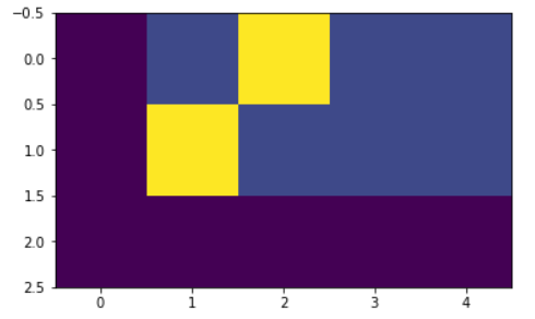
Examples of label smoothing ：

# Label smoothing Example 
crit = LabelSmoothing(5, 0, 0.4)  #  Set up a ϵ=0.4
predict = torch.FloatTensor([[0, 0.2, 0.7, 0.1, 0],
                             [0, 0.2, 0.7, 0.1, 0], 
                             [0, 0.2, 0.7, 0.1, 0]])
v = crit(Variable(predict.log()), 
         Variable(torch.LongTensor([2, 1, 0])))

# Show the target distributions expected by the system.
print(crit.true_dist)
plt.imshow(crit.true_dist)

tensor([[0.0000, 0.1333, 0.6000, 0.1333, 0.1333],
        [0.0000, 0.6000, 0.1333, 0.1333, 0.1333],
        [0.0000, 0.0000, 0.0000, 0.0000, 0.0000]])

Calculate the loss

class SimpleLossCompute:
    """  Simple calculation of the loss and parameter back propagation update training function  """
    def __init__(self, generator, criterion, opt=None):
        self.generator = generator
        self.criterion = criterion
        self.opt = opt
        
    def __call__(self, x, y, norm):
        x = self.generator(x)
        loss = self.criterion(x.contiguous().view(-1, x.size(-1)), 
                              y.contiguous().view(-1)) / norm
        loss.backward()
        if self.opt is not None:
            self.opt.step()
            self.opt.optimizer.zero_grad()
        return loss.data.item() * norm.float()

Optimizer

Adam Optimizer ,${\beta }_1=0.9、{\beta }_2=0.98$ and $ϵ=10^{-9}$, And use warmup Strategy adjustment learning rate ：

$$lr=d_{\text{model}}^{-0.5}\min ({\text{step\_num}}^{-0.5},\text{step\_num}\times {\text{warmup\_steps}}^{-1.5})$$

Use a fixed number of steps $\text{warmup\_steps}$ First, let the learning rate increase linearly （ Warm up ）, And then with $\text{step\_num}$ The increase in $\text{step\_num}$ Is proportional to the inverse square root of Gradually reduce the learning rate .

class NoamOpt:
    "Optim wrapper that implements rate."
    def __init__(self, model_size, factor, warmup, optimizer):
        self.optimizer = optimizer
        self._step = 0
        self.warmup = warmup
        self.factor = factor
        self.model_size = model_size
        self._rate = 0
        
    def step(self):
        "Update parameters and rate"
        self._step += 1
        rate = self.rate()
        for p in self.optimizer.param_groups:
            p['lr'] = rate
        self._rate = rate
        self.optimizer.step()
        
    def rate(self, step = None):
        "Implement `lrate` above"
        if step is None:
            step = self._step
        return self.factor * (self.model_size ** (-0.5) * min(step ** (-0.5), step * self.warmup ** (-1.5)))
        
def get_std_opt(model):
    return NoamOpt(model.src_embed[0].d_model, 2, 4000,
            torch.optim.Adam(model.parameters(), lr=0, betas=(0.9, 0.98), eps=1e-9))

The main adjustment is in $rate$ In this function , among

• $model\_size$ That is to say $d_{model}$
• $warmup$ That is to say $warmup\_steps$
• $factor$ It can be understood as the initial learning rate

The following describes the optimizer in Different model sizes （$model\_size$） and Different super parameters （$marmup$） value The learning rate in the case of （$lrate$） Curve for example .

# Three settings of the lrate hyperparameters.
opts = [NoamOpt(512, 1, 4000, None), 
        NoamOpt(512, 1, 8000, None),
        NoamOpt(256, 1, 4000, None)]
plt.plot(np.arange(1, 20000), [[opt.rate(i) for opt in opts] for i in range(1, 20000)])
plt.legend(["512:4000", "512:8000", "256:4000"])

Training

Next , We created a common training and scoring function to track losses . We pass in a loss calculation function defined above , It also handles parameter updates .

def run_epoch(data, model, loss_compute, epoch):
    start = time.time()
    total_tokens = 0.
    total_loss = 0.
    tokens = 0.

    for i , batch in enumerate(data):
        out = model(batch.src, batch.trg, batch.src_mask, batch.trg_mask)
        loss = loss_compute(out, batch.trg_y, batch.ntokens)

        total_loss += loss
        total_tokens += batch.ntokens
        tokens += batch.ntokens

        if i % 50 == 1:
            elapsed = time.time() - start
            print("Epoch %d Batch: %d Loss: %f Tokens per Sec: %fs" % (epoch, i - 1, loss / batch.ntokens, (tokens.float() / elapsed / 1000.)))
            start = time.time()
            tokens = 0

    return total_loss / total_tokens


def train(data, model, criterion, optimizer):
    """  Train and save models  """
    #  The initialization model is in dev The best on a set Loss Is a larger value 
    best_dev_loss = 1e5
    
    for epoch in range(EPOCHS):
        #  model training 
        model.train()
        run_epoch(data.train_data, model, SimpleLossCompute(model.generator, criterion, optimizer), epoch)
        model.eval()

        #  stay dev On the set loss assessment 
        print('>>>>> Evaluate')
        dev_loss = run_epoch(data.dev_data, model, SimpleLossCompute(model.generator, criterion, None), epoch)
        print('<<<<< Evaluate loss: %f' % dev_loss)
        
        #  If at present epoch The model of dev On set loss Better than the previous record loss Save the current model , And update the best loss value 
        if dev_loss < best_dev_loss:
            torch.save(model.state_dict(), SAVE_FILE)
            best_dev_loss = dev_loss
            print('****** Save model done... ******')       
            
        print()

Then you can train

#  Data preprocessing 
data = PrepareData(TRAIN_FILE, DEV_FILE)
src_vocab = len(data.en_word_dict)
tgt_vocab = len(data.cn_word_dict)
print("src_vocab %d" % src_vocab)
print("tgt_vocab %d" % tgt_vocab)

#  Initialize model 
model = make_model(
                    src_vocab, 
                    tgt_vocab, 
                    LAYERS, 
                    D_MODEL, 
                    D_FF,
                    H_NUM,
                    DROPOUT
                )

#  Training 
print(">>>>>>> start train")
train_start = time.time()
criterion = LabelSmoothing(tgt_vocab, padding_idx = 0, smoothing= 0.0)
optimizer = NoamOpt(D_MODEL, 1, 2000, torch.optim.Adam(model.parameters(), lr=0, betas=(0.9,0.98), eps=1e-9))

train(data, model, criterion, optimizer)
print(f"<<<<<<< finished train, cost {
      time.time()-train_start:.4f} seconds")

Model to predict

After training , Let's use the model to predict the effect ：

def greedy_decode(model, src, src_mask, max_len, start_symbol):
    """  Pass in a trained model , Forecast the specified data  """
    #  First use encoder Conduct encode
    memory = model.encode(src, src_mask)
    #  The initialization prediction content is 1×1 Of tensor, Fill in the opening character ('BOS') Of id, And will type Set to input data type (LongTensor)
    ys = torch.ones(1, 1).fill_(start_symbol).type_as(src.data)
    #  Traverse the length subscript of the output 
    for i in range(max_len-1):
        # decode The hidden layer representation is obtained 
        out = model.decode(memory, 
                           src_mask, 
                           Variable(ys), 
                           Variable(subsequent_mask(ys.size(1)).type_as(src.data)))
        #  Change the hidden representation to the words in the dictionary log_softmax The probability distribution represents 
        prob = model.generator(out[:, -1])
        #  Get the prediction word of the maximum probability of the current position id
        _, next_word = torch.max(prob, dim = 1)
        next_word = next_word.data[0]
        #  The character that predicts the current position id Spliced with previous predictions 
        ys = torch.cat([ys, 
                        torch.ones(1, 1).type_as(src.data).fill_(next_word)], dim=1)
    return ys


def evaluate(data, model):
    """  stay data Use the trained model to predict , Print model translation results  """
    #  Gradient clear 
    with torch.no_grad():
        #  stay data English data length traversal subscript 
        for i in range(len(data.dev_en)):
            #  Print the English sentence to be translated 
            en_sent = " ".join([data.en_index_dict[w] for w in data.dev_en[i]])
            print("\n" + en_sent)
            
            #  Print the corresponding Chinese sentence answer 
            cn_sent = " ".join([data.cn_index_dict[w] for w in data.dev_cn[i]])
            print("".join(cn_sent))
            
            #  Change the current word to id The English statement data represented by is converted to tensor, And put as DEVICE in 
            src = torch.from_numpy(np.array(data.dev_en[i])).long().to(DEVICE)
            #  Add one dimension 
            src = src.unsqueeze(0)
            #  Set up attention mask
            src_mask = (src != 0).unsqueeze(-2)
            #  Use the trained model decode forecast 
            out = greedy_decode(model, src, src_mask, max_len=MAX_LENGTH, start_symbol=data.cn_word_dict["BOS"])
            #  Initialize a list of words used to store the model translation results 
            translation = []
            #  Traverse the subscript of the translation output character （ Be careful ： Start Rune "BOS" The index of 0 Not traversal ）
            for j in range(1, out.size(1)):
                #  Get the output character of the current subscript 
                sym = data.cn_index_dict[out[0, j].item()]
                #  If the output character is not 'EOS' Terminator , Is added to the translation result list of the current statement 
                if sym != 'EOS':
                    translation.append(sym)
                #  Otherwise, the traversal is terminated 
                else:
                    break
            #  Print the Chinese sentence results of the model translation output 
            print("translation: %s" % " ".join(translation))

#  forecast 
#  Load model 
model.load_state_dict(torch.load(SAVE_FILE))
#  Start to predict 
print(">>>>>>> start evaluate")
evaluate_start  = time.time()
evaluate(data, model)
print(f"<<<<<<< finished evaluate, cost {
      time.time()-evaluate_start:.4f} seconds")

BOS look around . EOS
BOS  Four   It's about   see   see  . EOS
translation:  see  ！

BOS hurry up . EOS
BOS  catch   fast  ! EOS
translation:  fast   spot  ！

BOS keep trying . EOS
BOS  Following   To continue   No   force  . EOS
translation:  Following   To continue   No   force  .

BOS take it . EOS
BOS  take   go   Well  . EOS
translation:  Go to   take   Well  .

BOS birds fly . EOS
BOS  bird   class   fly   That's ok  . EOS
translation:  bird   class   fly   That's ok  .

BOS hurry up . EOS
BOS  fast   spot  ！ EOS
translation:  fast   spot  ！

BOS look there . EOS
BOS  see   that   in  . EOS
translation:  see   that   in   see   see  .

BOS how annoying ! EOS
BOS  really   Bother   people  . EOS
translation:  really   Bother   people  .

BOS get serious . EOS
BOS  recognize   really   spot  . EOS
translation:  recognize   really   spot  .

BOS once again . EOS
BOS  Again   One   Time  . EOS
translation:  Again   Time   One   Time  .

BOS stay sharp . EOS
BOS  Protect   a   police   Be vigilant  . EOS
translation:  Protect   a   police   Be vigilant  .

BOS i won ! EOS
BOS  I   win   了  . EOS
translation:  I   win   have to   了  .

BOS get away ! EOS
BOS  roll  ！ EOS
translation:  go   open  ！

BOS i resign . EOS
BOS  I   discharge   Discard  . EOS
translation:  I   discharge   Discard  .

BOS how strange ! EOS
BOS  really   p.   blame  . EOS
translation:  really   p.   blame  .
...

Reference resources

1. Explain profound theories in simple language Transformer
2. Greedy college courses