当前位置:网站首页>Construction of occupancy grid map
Construction of occupancy grid map
2022-06-25 07:35:00 【Ling Mountain】
grid map (occupancy grid map) structure
Reference:
1. Classification of maps

Scale map : With real physical dimensions , Such as grid map 、 Feature maps 、 Point cloud map , Commonly used in map construction 、 location 、SLAM、 Small scale path planning .
Topological map : No real physical size , It only represents the connectivity and distance of different places , Such as railway network , It is often used in large-scale robot path planning .
Semantic map : Labeled scale map ,SLAM And deep learning , Commonly used in human-computer interaction .
The scale map is supplemented , As shown in the figure below :
2. Occupy grid map construction algorithm
2.1 Why use the occupancy grid map building algorithm to build a map ?
Sensors for building raster maps ( Like a camera 、 Laser radar 、 Millimeter wave radar sensor ) There is noise , Popular said , Not necessarily .
for instance , Robots at different times in the same posture , The detection range of a fixed obstacle by lidar is inconsistent , One frame is 5 m 5m 5m, One frame is 5.1 m 5.1m 5.1m, Are we going to 5 m 5m 5m and 5.1 m 5.1m 5.1m All locations are marked as obstacles ? This is why the occupancy grid map construction algorithm is used .
2.2 What is the occupancy grid map construction algorithm ?
To solve this problem , We introduce Occupy the grid map (Occupancy Grid Map) The concept of . We rasterize the map , For each grid state, it either occupies , Or free , Or unknown ( The initialization state ).
On the introduction of occupation grid map construction algorithm 、 deduction 、 Evolution , It can be obtained from the following formula :
For each grid , We use it p ( s = 1 ) p(s=1) p(s=1) To express Free The probability of States , We use it p ( s = 0 ) p(s=0) p(s=0) To express Occupied The probability of States , The sum of the two is 1 1 1.
Use two values to represent the state of a grid , It's a bit wrong. , So we introduce the ratio of the two to represent the state of the grid :
Odd ( s ) = p ( s = 1 ) p ( s = 0 ) \operatorname{Odd}(s)=\frac{p(s=1)}{p(s=0)} Odd(s)=p(s=0)p(s=1)
When lidar measurements are observed (z~{0,1}) After arrival , The relevant grid needs to update the grid status O d d ( s ) Odd(s) Odd(s).
Suppose the lidar measurements come before , The status of the grid is O d d ( s ) Odd(s) Odd(s), After coming , The status of the update grid is :
O d d ( s ∣ z ) = p ( s = 1 ∣ z ) p ( s = 0 ∣ z ) Odd(s \mid z)=\frac{p(s=1 \mid z)}{p(s=0 \mid z)} Odd(s∣z)=p(s=0∣z)p(s=1∣z)
This expression is similar to conditional probability , It means that z z z The state of the grid under occurrence conditions .
According to Bayes formula, the following two formulas are obtained :
p ( s = 1 ∣ z ) = p ( z ∣ s = 1 ) p ( s = 1 ) p ( z ) p ( s = 0 ∣ z ) = p ( z ∣ s = 0 ) p ( s = 0 ) p ( z ) \begin{array}{l} p(s=1 \mid z)=\frac{p(z \mid s=1) p(s=1)}{p(z)} \\ p(s=0 \mid z)=\frac{p(z \mid s=0) p(s=0)}{p(z)} \end{array} p(s=1∣z)=p(z)p(z∣s=1)p(s=1)p(s=0∣z)=p(z)p(z∣s=0)p(s=0)
Substitute the above two formulas into O d d ( s ) Odd(s) Odd(s) after , We come to the conclusion that :
Odd ( s ∣ z ) = p ( s = 1 ∣ z ) p ( s = 0 ∣ z ) Odd ( s ∣ z ) = p ( z ∣ s = 1 ) p ( s = 1 ) p ( z ∣ s = 0 ) p ( s = 0 ) Odd ( s ∣ z ) = p ( z ∣ s = 1 ) p ( z ∣ s = 0 ) ∗ p ( s = 1 ) p ( s = 0 ) Odd ( s ∣ z ) = p ( z ∣ s = 1 ) p ( z ∣ s = 0 ) ∗ Odd ( s ) \begin{array}{l} \operatorname{Odd}(s \mid z)=\frac{p(s=1 \mid z)}{p(s=0 \mid z)} \\ \operatorname{Odd}(s \mid z)=\frac{p(z \mid s=1) p(s=1)}{p(z \mid s=0) p(s=0)} \\ \operatorname{Odd}(s \mid z)=\frac{p(z \mid s=1)}{p(z \mid s=0)} * \frac{p(s=1)}{p(s=0)} \\ \operatorname{Odd}(s \mid z)=\frac{p(z \mid s=1)}{p(z \mid s=0)} * \operatorname{Odd}(s) \end{array} Odd(s∣z)=p(s=0∣z)p(s=1∣z)Odd(s∣z)=p(z∣s=0)p(s=0)p(z∣s=1)p(s=1)Odd(s∣z)=p(z∣s=0)p(z∣s=1)∗p(s=0)p(s=1)Odd(s∣z)=p(z∣s=0)p(z∣s=1)∗Odd(s)
here , Let's take logarithms on both sides of the above equation to get : The grid state representation changes again , The box log Odd ( s ) \log \operatorname{Odd}(s) logOdd(s) Indicates the state of a grid .
log Odd ( s ∣ z ) = log p ( z ∣ s = 1 ) p ( z ∣ s = 0 ) + log Odd ( s ) \log \operatorname{Odd}(s \mid z)=\log \frac{p(z \mid s=1)}{p(z \mid s=0)}+\log \operatorname{Odd}(s) logOdd(s∣z)=logp(z∣s=0)p(z∣s=1)+logOdd(s)
In this case, the only item containing the measured value is log p ( z ∣ s = 1 ) p ( z ∣ s = 0 ) \log \frac{p(z \mid s=1)}{p(z \mid s=0)} logp(z∣s=0)p(z∣s=1) 了 . We call this ratio the model of the measured value .
log p ( z ∣ s = 1 ) p ( z ∣ s = 0 ) \log \frac{p(z \mid s=1)}{p(z \mid s=0)} logp(z∣s=0)p(z∣s=1) There are only two options for l o f r e e lofree lofree and l o o c c u looccu looccu, Because there are only two kinds of laser radar observations on a grid : Occupy and idle .
lofree = log p ( z = 0 ∣ s = 1 ) p ( z = 0 ∣ s = 0 ) looccu = log p ( z = 1 ∣ s = 1 ) p ( z = 1 ∣ s = 0 ) \begin{array}{l} \text { lofree }=\log \frac{p(z=0 \mid s=1)}{p(z=0 \mid s=0)} \\ \text { looccu }=\log \frac{p(z=1 \mid s=1)}{p(z=1 \mid s=0)} \end{array} lofree =logp(z=0∣s=0)p(z=0∣s=1) looccu =logp(z=1∣s=0)p(z=1∣s=1)
here , If we use log Odd ( s ) \log \operatorname{Odd}(s) logOdd(s) To represent the grid s s s The state of S S S Words , Our update rule is further simplified to :
S + = S − + log p ( z ∣ s = 1 ) p ( z ∣ s = 0 ) S^{+}=S^{-}+\log \frac{p(z \mid s=1)}{p(z \mid s=0)} S+=S−+logp(z∣s=0)p(z∣s=1)
among , S + S^{+} S+ and S − S^{-} S− Represents the grid after and before the measured value respectively s s s The state of .
Besides , The initial state of a grid S i n i t S_{init} Sinit by : The default probability of free and occupied grids is 0.5 0.5 0.5.
S init = log 0 d d ( s ) = log p ( s = 1 ) p ( s = 0 ) = log 0.5 0.5 = 0 S_{\text {init }}=\log 0 d d(s)=\log \frac{p(s=1)}{p(s=0)}=\log \frac{0.5}{0.5}=0 Sinit =log0dd(s)=logp(s=0)p(s=1)=log0.50.5=0
here , After such modeling , To update the state of a grid, simply add it :
S + = S − + lofree or S + = S − + looccu \begin{array}{c} S^{+}=S^{-}+\text {lofree } \\ \text { or } \\ S^{+}=S^{-}+\text {looccu } \end{array} S+=S−+lofree or S+=S−+looccu
2.3 Take an example to verify the occupancy grid map construction algorithm
First , We assume that l o o c c u = 0.9 looccu = 0.9 looccu=0.9, l o f r e e = − 0.7 lofree = -0.7 lofree=−0.7. that , Obvious , The larger the value of a grid state , The more it means that the grid is occupied ; On the contrary, the smaller the value , It means that the grid is idle .( This also solves the problem of lidar observation value proposed in the previous article " Not necessarily " The problem of )
The above figure shows the process of updating the map with two laser scanning data . In the result , The darker the color, the more the grid is free , The lighter the color, the more occupied it is . Here we should distinguish between the commonly used lasers SLAM Map in algorithm , It's just the different ways of expression , There is no right or wrong .
3. How to build a grid map from lidar data ?
3.1 The core basis of the algorithm
A conclusion drawn from the whole article is shown in the figure below , It is assumed that l o f r e e lofree lofree and l o o c c u looccu looccu Is the determined value , In general, one positive and one negative .
S + = S − + lofree or S + = S − + looccu \begin{array}{c} S^{+}=S^{-}+\text {lofree } \\ \text { or } \\ S^{+}=S^{-}+\text {looccu } \end{array} S+=S−+lofree or S+=S−+looccu
then , We judge by the lidar data grid : If the grid is determined to be idle , Just execute the above formula ; If the decision grid is occupied , Just execute the following formula . After many frames of lidar data , Each grid stores a value , At this point, we can set our own threshold to compare with this value , To determine the final state of the grid .
3.2 Algorithm input data
Lidar packet ( Each scan point contains an angle ( Counterclockwise is positive ) And distance , Each frame of laser data contains several scanning points , The lidar data packet contains several frames of lidar data )
Robot pose data packet ( Each pose contains the robot position and heading angle in the world coordinate system , Initial heading angle and world coordinate system X The axes coincide in the positive direction , Counterclockwise is positive )
Map parameters ( You need to build the height and width of the map , Starting point for building a map , l o f r e e lofree lofree and l o o c c u looccu looccu Set value of , The resolution of the map )
It is assumed that the lidar coordinate system coincides with the robot coordinate system .
3.3 Algorithm steps
Here, the first frame of lidar processing is taken as an example , From top to bottom :
- Read a frame of lidar data and the corresponding robot pose
// Acquire the lidar of each frame 、 Robot pose data
GeneralLaserScan scan = scans[i];
Eigen::Vector3d robotPose = robot_poses[i];
- Calculate the grid sequence number of the robot position in this frame
// Get the grid sequence number of the robot pose in this frame
GridIndex robotIndex = ConvertWorld2GridIndex(robotPose(0),robotPose(1));
That is, from the world coordinate system to the grid coordinate system , Each grid number has x x x, y y y Two figures . This is related to the resolution of the map , for instance : The map resolution is 0.05 0.05 0.05, That is to say 1 m 1m 1m use 20 20 20 A grid represents .
for example : Robot position in the world coordinate system (1,1) Corresponding to the grid coordinate system (20,20).
Be careful : The world coordinate system is distinguished from the pixel coordinate system , Between them y Opposite axis direction , Everything else is the same , The pixel coordinate system used for map display ( Grid coordinate system ).
- Traverse all scanning points of the lidar data of this frame and perform the following operations
Calculate the grid serial number of the grid in the pixel coordinate system in each laser click :
// Define the world coordinate system here world_x, Not a real world coordinate system , It's a pixel coordinate system ,y The axis is opposite to the real world coordinate system , This is a laser_y Reason for minus sign
double laser_x =   dist * cos(theta + angle);
double laser_y =  -dist * sin(theta + angle);

// Obtain the laser scanning point , In the world coordinate system ( Pixel coordinate system ) The location of
double world_x = laser_x + robotPose(0);
double world_y = laser_y + robotPose(1);

// The position of the laser scanning point in the world coordinate system , Convert to grid sequence number
GridIndex mapIndex = ConvertWorld2GridIndex(world_x,world_y);
 From the grid sequence number of the current robot pose to the grid sequence number of the laser scanning point , Find out all the free grid numbers :
// From the grid number of the robot to the grid number of the laser scanning point
// Purpose : Find a free grid of paths between two points , Save the grid serial number into std::vector<GridIndex> in
std::vector<GridIndex> freeIndex = TraceLine(robotIndex.x,robotIndex.y,mapIndex.x,mapIndex.y);

- Traverse all idle grids to update the idle grid status :
data += mapParams.log_free;//log_free=-1,data Will be smaller
- Update the grid status in the laser scanning click :
data += mapParams.log_occ;//log_occ=2,data It's going to get bigger
4. Occupy grid map construction algorithm c++ Realization
Share the core code here , Specific algorithm function package , Available in the public number : Xiaobai learns mobile robot , send out : grid map , You can get .
// Occupy grid map construction algorithm
// Input lidar data and robot pose data
// Purpose : By traversing all frame data , by pMap[] Each passing through the free grid or hitting the grid is assigned a new value , There is a calculation method in the middle , That is to say, the theoretical realization of grid map construction
void OccupanyMapping(std::vector<GeneralLaserScan>& scans,std::vector<Eigen::Vector3d>& robot_poses)
{

  std::cout <<"Scans Size:"<<scans.size()<<std::endl;
  std::cout <<"Poses Size:"<<robot_poses.size()<<std::endl;

  // Traverse all frames of lidar data
  for(int i = 0; i < scans.size();i++)
  {

    // Acquire the lidar of each frame 、 Robot pose data
    GeneralLaserScan scan = scans[i];
    Eigen::Vector3d robotPose = robot_poses[i];

    // Get the grid sequence number of the robot pose in this frame
    GridIndex robotIndex = ConvertWorld2GridIndex(robotPose(0),robotPose(1));

    // Determine the grid sequence number of the robot pose in this frame , Whether it is within the range of the grid map you set
    if(isValidGridIndex(robotIndex) == false) continue;

    // Traverse all scanning points of this frame of lidar data
    for(int id = 0; id < scan.range_readings.size();id++)
    {

      // Take out the distance and angle of the laser radar scanning point
      double dist = scan.range_readings[id];
      double angle = scan.angle_readings[id];
      // Remove abnormal data , Skip the loop , Do not deal with
      if(std::isinf(dist) || std::isnan(dist)) continue;
      // Robot heading angle , robot x Axis and world coordinate system x Included angle of shaft
      double theta = robotPose(2);

      // After the rotation ( And the world coordinate system ( Pixel coordinate system ) parallel ) The coordinates in the lidar coordinate system x,y
      // I don't understand why at first laser_y To add a minus sign
      // Make sure that the angle of lidar data changes counterclockwise
      // Define the heading angle of the robot and the world coordinate system x The axis changes counterclockwise
      // Define the world coordinate system here world_x, Not a real world coordinate system , It's a pixel coordinate system ,y The axis is opposite to the real world coordinate system , This is a laser_y Reason for minus sign
      double laser_x =   dist * cos(theta + angle);
      double laser_y =  -dist * sin(theta + angle);

      // Obtain the laser scanning point , In the world coordinate system ( Pixel coordinate system ) The location of
      double world_x = laser_x + robotPose(0);
      double world_y = laser_y + robotPose(1);

      // The position of the laser scanning point in the world coordinate system , Convert to grid sequence number
      GridIndex mapIndex = ConvertWorld2GridIndex(world_x,world_y);

      // Judge the grid serial number of the laser scanning point , Whether to use the grid map set by yourself 900x900 Within the scope of , If not, skip
      if(isValidGridIndex(mapIndex) == false)continue;

      // From the grid number of the robot to the grid number of the laser scanning point
      // Purpose : Find a free grid of paths between two points , Save the grid serial number into std::vector<GridIndex> in
      std::vector<GridIndex> freeIndex = TraceLine(robotIndex.x,robotIndex.y,mapIndex.x,mapIndex.y);

      // Traverse all the free grids through which the scanning laser point passes
      for(int k = 0; k < freeIndex.size();k++)
      {

        GridIndex tmpIndex = freeIndex[k];
        // The grid sequence number of the free grid , Convert to array ordinal , This array is used to store the data of each grid
        int linearIndex = GridIndexToLinearIndex(tmpIndex);
        // Take out the data represented by the grid
        int data = pMap[linearIndex];
        // According to the grid idle rule , perform data += mapParams.log_free;
        if(data > 0)// Default data=50
          data += mapParams.log_free;//log_free=-1,data Will be smaller
        else
          data = 0;
        // Assign a new value to the free grid , The minimum is 0
        pMap[linearIndex] = data;
      }
      // Update the grid in the laser scanning point set ,
      int tmpIndex = GridIndexToLinearIndex(mapIndex);
      int data = pMap[tmpIndex];
      // According to the grid hit rule , perform data += mapParams.log_occ;
      if(data < 100)// Default data=50
        data += mapParams.log_occ;//log_occ=2,data It's going to get bigger
      else
        data = 100;
      // Assign a new value to the hit grid , Maximum 100
      pMap[tmpIndex] = data;
      // Come here , For a laser scanning data in a pose, the idle grid passed by and the hit grid pMap Reassigned
    }
    // Come here , The free grid and hit grid of a frame of laser scanning data in a pose are re assigned
  }
  // Come here , The free grid and hit grid passed by all frames of laser scanning data are re assigned
}
边栏推荐
- Design a MySQL table for message queue to store message data
- MySQL (12) -- Notes on changing tables
- Sichuan Tuwei ca-if1051 can transceiver has passed aec-q100 grade 1 certification
- MySQL - definition and assignment of variables
- Explain distributed raft with dynamic diagram
- shell小技巧(一百三十四)简单的键盘输入记录器
- PI Ziheng embedded: This paper introduces the multi-channel link mode of i.mxrt timer pit and its application in coremark Test Engineering
- Kube scheduler source code analysis (1) - initialization and startup analysis
- 线程状态变化涉及哪些常用 API
- MySQL(十二)——更改表的备注
猜你喜欢
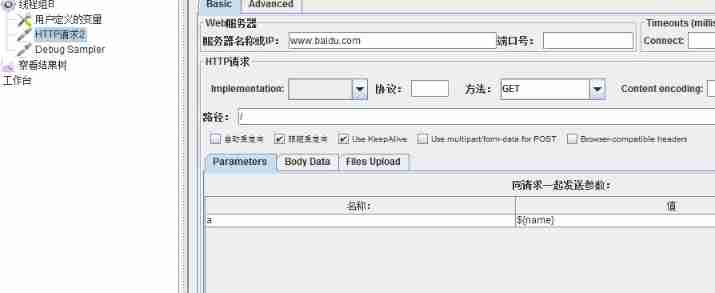
JMeter introduction practice ----- use of global variables and local variables

VectorDraw Developer Framework 10.10

Zhugeliang vs pangtong, taking distributed Paxos

【批处理DOS-CMD命令-汇总和小结】-应用程序启动和调用、服务和进程操作命令(start、call、)

Operate cnblogs metaweblog API
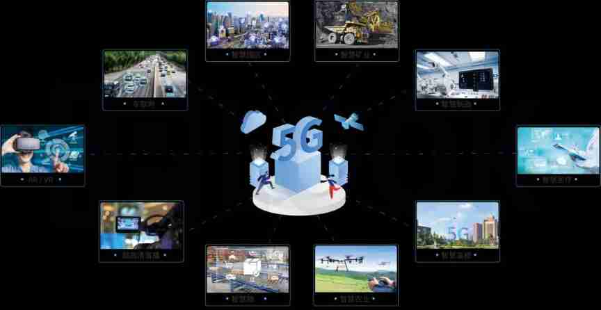
5g private network market is in full swing, and it is crucial to solve deployment difficulties in 2022

韩信大招:一致性哈希

Explain distributed raft with dynamic diagram

线程状态变化涉及哪些常用 API

为什么要“除夕”,原来是内存爆了!
随机推荐
What common APIs are involved in thread state changes
The perfect presentation of Dao in the metauniverse, and platofarm creates a farm themed metauniverse
MySQL (12) -- Notes on changing tables
Orcad Schematic常用功能
[C language] add separator to string
Tempest HDMI leak receive 1
TEMPEST HDMI泄漏接收 1
Operate cnblogs metaweblog API
Mysql database import SQL file display garbled code
用动图讲解分布式 Raft
[batch dos-cmd command - summary and summary] - external command -cmd download command and packet capture command (WGet)
高考志愿填报,为啥专业最后考虑?
How comfortable it is to use Taijiquan to talk about distributed theory!
How is the network connected?
Why "New Year's Eve", the original memory burst!
What is the new business model of Taishan crowdfunding in 2022?
为什么要“除夕”,原来是内存爆了!
Introduction to Sichuan Tuwei ca-is3082w isolated rs-485/rs-422 transceiver
Common functions of OrCAD schematic
【批处理DOS-CMD命令-汇总和小结】-CMD窗口的设置与操作命令(cd、title、mode、color、pause、chcp、exit)