当前位置:网站首页>Digital image processing Chapter 4 - frequency domain filtering
Digital image processing Chapter 4 - frequency domain filtering
2022-07-27 05:57:00 【Hai Ou Wan Ramen】
Catalog
4.1.3 Impulse and its sampling characteristics
4.1.4 Fourier transform of continuous variable function
4.2 Sampling and Fourier transform of sampling function
4.2.2 Fourier transform of sampling function
4.3 Discrete Fourier transform of single variable (DFT)
4.3.1 From the continuous transformation of the sampled function DFT
4.4 Expansion of the function of two variables
4.4.1 Two dimensional impulse and its sampling
4.4.2 Two dimensional continuous Fourier transform pair
4.4.3 Two dimensional sampling and two dimensional sampling theorem
4.4.4 Two dimensional discrete Fourier transform and its inverse transform
4.5 Some properties of two-dimensional discrete Fourier transform
4.5.1 The relationship between space and frequency interval
4.5.2 Translation and rotation
4.5.5 Fourier spectrum and phase angle
4.5.6 Two dimensional convolution theorem
4.5.7 Summary of the properties of two-dimensional discrete Fourier transform
4.6 Basis of frequency domain filtering
4.6.1 Basis of frequency domain filtering
4.6.2 Summary of filtering steps in frequency domain
4.6.3 Correspondence between spatial and frequency domain filtering
4.7 Use frequency table and filter to smooth the image
4.7.2 Butterworth low pass filter
4.7.3 Gaussian low pass filter
4.8 Sharpen the image using a frequency domain filter
4.8.2 Butterworth high pass filter
4.8.3 Gaussian high pass filter
4.8.4 Laplace operator in frequency domain
4.8.5 Passivation template 、 High lift filtering and high frequency emphasis filtering
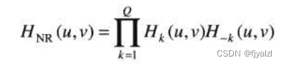
4.9.1 Band stop filter and band pass filter
4.1 Basic concepts
4.1.1 The plural
The plural C The definition is as follows :

In style ,R and I Is the set of real Numbers ,j Is one equal to -1 The imaginary number of the square root of , namely ![]() .R The real part of a complex number ,I Represents the imaginary part of a complex number .
.R The real part of a complex number ,I Represents the imaginary part of a complex number .
The real number is I=0 Subset of the complex number of . The plural C The conjugate of is expressed as C*, Its definition is
![]()
Euler formula :
![]()
Euler formula complex number representation in polar coordinates :
![]()
4.1.2 Fourier series
With period T A continuous variable of t The periodic function of f(t) It can be described as the sum of sine and cosine multiplied by appropriate coefficients . This sum is Fourier series

In style ,
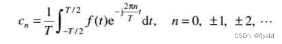
It's a coefficient .
4.1.3 Impulse and its sampling characteristics
An impulse has a so-called sampling characteristic with respect to the following integral :

hypothesis f(t) stay t=0 The place is continuous , The sampling characteristics get the function f(t) The value at the impulse position . A more general description of sampling characteristics involves being located at any point t0 Impulse of , Expressed as ![]() . In this case, the sampling characteristic becomes :
. In this case, the sampling characteristic becomes :

The sampling characteristics of discrete variables have the following forms :

More generally, use location x=x0 Discrete impulse at

An impulse string is defined as an infinite number of discrete periodic impulse elements △T The sum of the :

4.1.4 Fourier transform of continuous variable function
Continuous variable t The continuous function of f(t) The Fourier transform of is defined by :

It can also be written as

![]()
Using Euler's formula , The second formula can be expressed as :

4.1.5 Convolution
Convolution is defined as follows

Convolution theorem :
![]()
![]()
4.2 Sampling and Fourier transform of sampling function
4.2.1 sampling
After sampling, the function is expressed as :

Each component of this formula is determined by the impulse position f(t) Value of weighted impulse . Each sample value is stimulated by the weighted impulse “ Strength ” give , We can get it by integrating . in other words , Any sampled value in the sequence fk Given by the following formula :
![]()

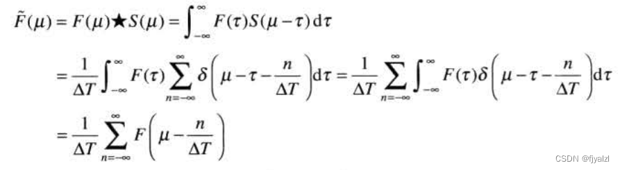
4.2.2 Fourier transform of sampling function
![]()
among ,

available F(μ) and S(μ) Convolution of :
4.3 Discrete Fourier transform of single variable (DFT)
4.3.1 From the continuous transformation of the sampled function DFT

Fourier forward transform and inverse transform are infinite periodic , Its period is M, namely :
![]()
and
![]()
4.4 Expansion of the function of two variables
4.4.1 Two dimensional impulse and its sampling
Two continuous variables t and z The impulse of is defined as the following form :

For two-dimensional discrete variables , Its impulse is defined as

The sampling characteristics are
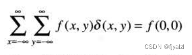
For coordinates (x0,y0) External impulse , The sampling characteristics are

4.4.2 Two dimensional continuous Fourier transform pair
Make f(t,z) Are two continuous variables t and z The continuous function of . Then its two-dimensional continuous Fourier transform pair is given by the following two expressions :

In style ,μ and v It's a frequency variable . When it comes to images ,t and z Interpreted as continuous spatial variables . Just like the one-dimensional case , Variable μ and v The domain of defines the continuous frequency domain .
4.4.3 Two dimensional sampling and two dimensional sampling theorem
Sampling function can be used for two-dimensional sampling ( Two dimensional impulse string ) modeling :

4.4.4 Two dimensional discrete Fourier transform and its inverse transform
Two dimensional Fourier transform (DFT) by :

Reverse transformation (IDFT) by :

4.5 Some properties of two-dimensional discrete Fourier transform
4.5.1 The relationship between space and frequency interval
Suppose for continuous functions f(t,z) Sampling generates a digital image f(x,y), It is divided into t and z Direction taken MxN Composed of samples . Make △T and △Z Represents the interval between samples . that , The intervals between the corresponding discrete frequency domain variables are respectively determined by

give . The interval between samples in frequency domain is inversely proportional to the interval between spatial samples and the number of samples .
4.5.2 Translation and rotation
Translation properties :

4.5.3 periodic
Two dimensional Fourier transform and its inverse transform are used in u Direction and v The direction is infinitely periodic

4.5.4 symmetry
Any real function or complex function w(x,y) Can be expressed as an odd part and an even part ( Each of them can be a real part or an imaginary part ) And :
![]()
among , The even and odd parts are defined as follows :
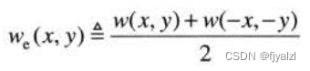
Even functions are symmetric , Odd functions are antisymmetric .
4.5.5 Fourier spectrum and phase angle
Use polar coordinates to represent two-dimensional DFT:

The range
![]()
It is called Fourier spectrum ( Or spectrum ), and

It is called phase angle .
The power spectrum is defined as
![]()
R and I Namely F(u,v) The real part and the virtual part of , also , All calculations are directly on discrete variables u=0,1,2,...,M-1 and v=0,1,2,...,N-1 Conduct .![]()
Fourier transform of real function is conjugate symmetric , This shows that the spectrum is even symmetric about the origin :
![]()
The phase angle is odd symmetric about the origin :
![]()
It points out the zero frequency term and f(x,y) Is proportional to the average of , Thus there are
![]()
4.5.6 Two dimensional convolution theorem
Two dimensional cyclic convolution expression :

The following expression of two-dimensional convolution is given :

4.5.7 Summary of the properties of two-dimensional discrete Fourier transform


Code implementation :
import os
import numpy as np
import cv2
import matplotlib.pyplot as plt
plt.rcParams['font.sans-serif'] = ['SimHei']
plt.rcParams['axes.unicode_minus'] = False

def put(path):
    img = cv2.imread(path, 1)
    # img = cv2.imread(os.path.join(base, path), 1)
    img = cv2.cvtColor(img, cv2.COLOR_BGR2GRAY)
    rows, cols = img.shape[:2]
    #  The Fourier transform
    dft = cv2.dft(np.float32(img), flags=cv2.DFT_COMPLEX_OUTPUT)
    #  Move the low frequency of the spectrum from the top left to the center
    dft_shift = np.fft.fftshift(dft)
    #  Spectrum image dual channel complex conversion to 0-255 Section
    res1 = 20 * np.log(cv2.magnitude(dft_shift[:, :, 0], dft_shift[:, :, 1]))
    #  Inverse Fourier transform
    ishift = np.fft.ifftshift(dft_shift)
    iimg = cv2.idft(ishift)
    res2 = cv2.magnitude(iimg[:, :, 0], iimg[:, :, 1])
    #  Image rotates clockwise 60 degree
    M = cv2.getRotationMatrix2D((cols / 2, rows / 2), -60, 1)
    rot = cv2.warpAffine(img, M, (rows, cols))
    #  The Fourier transform
    dft3 = cv2.dft(np.float32(rot), flags=cv2.DFT_COMPLEX_OUTPUT)
    dft_shift3 = np.fft.fftshift(dft3)
    res3 = 20 * np.log(cv2.magnitude(dft_shift3[:, :, 0], dft_shift3[:, :, 1]))
    #  Inverse Fourier transform
    ishift3 = np.fft.ifftshift(dft_shift3)
    iimg3 = cv2.idft(ishift3)
    res4 = cv2.magnitude(iimg3[:, :, 0], iimg3[:, :, 1])

    #  The image shifts to the right
    H = np.float32([[1, 0, 200], [0, 1, 0]])
    tra = cv2.warpAffine(img, H, (rows, cols))
    #  The Fourier transform
    dft2 = cv2.dft(np.float32(tra), flags=cv2.DFT_COMPLEX_OUTPUT)
    dft_shift2 = np.fft.fftshift(dft2)
    res5 = 20 * np.log(cv2.magnitude(dft_shift2[:, :, 0], dft_shift2[:, :, 1]))
    #  Inverse Fourier transform
    ishift2 = np.fft.ifftshift(dft_shift2)
    iimg2 = cv2.idft(ishift2)
    res6 = cv2.magnitude(iimg2[:, :, 0], iimg2[:, :, 1])
    #  Output results
    plt.rcParams['font.sans-serif'] = ['SimHei']
    plt.subplot(331), plt.imshow(img, plt.cm.gray), plt.title(' Original gray image '),plt.axis('off')
    plt.subplot(332),plt.imshow(res1,plt.cm.gray),plt.title(' The Fourier transform '),plt.axis('off')
    plt.subplot(333),plt.imshow(res2,plt.cm.gray),plt.title(' Inverse Fourier transform '),plt.axis('off')
    plt.subplot(334),plt.imshow(rot,plt.cm.gray),plt.title(' Image rotation '),plt.axis('off')
    plt.subplot(335),plt.imshow(res3,plt.cm.gray),plt.title(' The Fourier transform '),plt.axis('off')
    plt.subplot(336),plt.imshow(res4,plt.cm.gray),plt.title(' Inverse Fourier transform '),plt.axis('off')
    plt.subplot(337),plt.imshow(tra,plt.cm.gray),plt.title(' Image translation '),plt.axis('off')
    plt.subplot(338),plt.imshow(res5,plt.cm.gray),plt.title(' The Fourier transform '),plt.axis('off')
    plt.subplot(339),plt.imshow(res6,plt.cm.gray),plt.title(' Inverse Fourier transform '),plt.axis('off')

    # plt.savefig('1.new.jpg')
    plt.show()

#  Processing function , To pass in the path
put(r'G:\4.png')

4.6 Basis of frequency domain filtering
4.6.1 Basis of frequency domain filtering
Frequency domain filtering consists of modifying the Fourier transform of an image and then calculating its inverse transform to obtain the processed result . thus , Given a size of MxN Digital image of , The basic filtering formula of interest has the following form :
![]()
among ,![]() yes IDFT,F(u,v) It's the input image f(x,y) Of DFT,H(u,v) Is the filter function ( filter 、 Transfer function ),g(x,y) It's filtered ( Output ) Images . function F,H and g Is the same size as the input image MxN array .
yes IDFT,F(u,v) It's the input image f(x,y) Of DFT,H(u,v) Is the filter function ( filter 、 Transfer function ),g(x,y) It's filtered ( Output ) Images . function F,H and g Is the same size as the input image MxN array .
We think that the high frequency is attenuated and passes through the low frequency filter H(u,v)( It is approximately called a low-pass filter ) Will blur an image , Filters with opposite characteristics ( Called high pass filter ) Will enhance sharp details , But it will lead to the reduction of image contrast . Adding a small constant to the filter will not affect the sharpness , But it does prevent the elimination of DC terms , And keep the tone .
4.6.2 Summary of filtering steps in frequency domain
1. Given a size of MxN The input image of f(x,y), The filling parameters can be obtained P and Q. Typically , We choose P=2M and Q=2N. 2、 Yes f(x,y) Add the necessary quantity 0, The formation size is P×Q Fill image of fp(x,y)
3、 use (-1)^(x+y) multiply fp(x,y), Move to its transformation center .
4、 computational procedure 3 Discrete Fourier transform of image in (DFT), obtain F(u,v)
5、 Generate a filter function H(u,v), Its size is P×Q, The center is at the center of the image . Multiply the array to form a product
G(u,v)=H(u,v)F(u,v).
6、 Get the processed image : Inverse Fourier transform , And only select the real part , obtain gp(x,y)
7、 from gp(x,y) Extracted at the upper left quadrant of M×N Area , Get the final processing result g(x,y).
4.6.3 Correspondence between spatial and frequency domain filtering
The link between spatial domain and frequency domain filtering is convolution theorem . Given a spatial filter , The frequency domain representation of the spatial filter can be obtained by the Fourier forward transform . contrary , Follow its similar analysis and convolution theorem , Inverse transform of frequency domain filter , Filter corresponding to spatial domain . The two filters form a Fourier transform pair :
![]()
among ,h(x,y) Is a spatial filter . Because the filter can be obtained by the corresponding response of a frequency domain filter to an impulse , therefore h(x,y) Sometimes called H(u,v) Pulse response of . also , Because all values in the discrete implementation of the above formula are finite , Such a filter is called finite impulse response (FIR) filter .
Gaussian filter in frequency domain :
![]()
The corresponding filter in the spatial domain is obtained by its inverse transformation :
![]()
(1) They are a Fourier transform pair , Both components are Gaussian and real functions , This is convenient for analysis . At the same time, Gaussian curve is very intuitive , And easy to operate . (2) Functions behave as reciprocal . When H(u) When there is a wide shape (![]() ),h(x) It has a narrow shape , also , vice versa . in fact , When the value approaches infinity ,H(u) Close to a constant function , also h(x) Approaching an impulse , This means that filtering is not possible in both the frequency domain and the spatial domain .
),h(x) It has a narrow shape , also , vice versa . in fact , When the value approaches infinity ,H(u) Close to a constant function , also h(x) Approaching an impulse , This means that filtering is not possible in both the frequency domain and the spatial domain .
4.7 Use frequency table and filter to smooth the image
This part mainly introduces various filtering techniques in the frequency domain , The first is to introduce the low-pass filter , Low pass filter is mainly used to blur the image , Three types of low-pass filters are mainly introduced : Ideal filter / Butterworth low pass filter and Gauss low pass filter . High pass filter is mainly used to sharpen the image , Highlight edge features
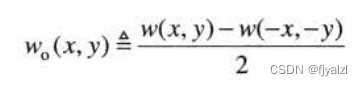
4.7.1 Ideal low pass filter
Take the origin as the center of the circle 、 With D0 Is the radius of the garden , Pass through all frequencies without attenuation , And outside the circle “ Cut off the ” Two dimensional low-pass filter of all frequencies , It is called ideal low-pass filter (ILPF); It is determined by the following function :

among D0 Is a normal number ,D(u,v) Is the midpoint of the frequency domain (u,v) Distance from the center of the rectangle in the frequency domain , namely
![]()

The filtering result is shown in the figure
Obvious ringing characteristics can be observed .IPLE The fuzziness and ringing characteristics of can be explained by convolution theorem .
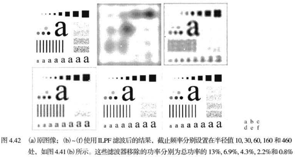
4.7.2 Butterworth low pass filter
The cut-off frequency is located at the distance from the origin D0 Situated n Order Butterworth low pass filter (BLPF) The transfer function of is defined as


It is obvious that the transition is smooth on the edge of black and white , In perspective 0 and 1 The transition is also smooth . The filtering results are as follows :

There is no obvious ringing effect in the figure . 、
4.7.3 Gaussian low pass filter
The two-dimensional form of the filter is given by the following formula :
![]()
Gaussian low pass filter (GLPF) The inverse Fourier transform of is also Gaussian , There will be no ringing .


4.8 Sharpen the image using a frequency domain filter
Because the sharp changes of edges and other grayscale are related to high-frequency components , Therefore, image sharpening can be achieved by high pass filtering in the frequency domain , High pass filtering will attenuate the low-frequency components in the Fourier transform without disturbing the high-frequency information .
A high pass filter is obtained from a given low-pass filter with the following formula :
![]()
among HLP(u,v) Is the transfer function of the low-pass filter . in other words , The frequency attenuated by the low-pass filter can pass through the high pass filter , vice versa .
4.8.1 Ideal high pass filter
A two-dimensional ideal high pass filter (IHPF) Defined as

among D0 Is the cut-off frequency .IHPF And ILPF Is relative , under these circumstances ,IHPF Take the radius as D0 All frequencies in the park are set to zero , And pass through all frequencies outside the circle without attenuation . Like ILPF like that ,IHPF It is also physically impossible ,IHPF It can be used to explain ringing and other phenomena in the spatial domain .
4.8.2 Butterworth high pass filter
The cut-off frequency is D0 Of n Step Butterworth high pass filter (BHPF) Defined as

4.8.3 Gaussian high pass filter
The cut-off frequency is at a distance of D0 Gaussian high pass filter (GHPF) The transfer function of is given by :

4.8.4 Laplace operator in frequency domain
Laplace operator can be realized in frequency domain by using the following filter :
![]()
perhaps , About the center of the frequency rectangle , Use the following filter :
![]()
The Laplace image is obtained by the following formula :
![]()
among ,F(u,v) yes f(x,y) The Fourier transform of . Enhancements can be achieved using the following formula :
![]()
4.8.5 Passivation template 、 High lift filtering and high frequency emphasis filtering
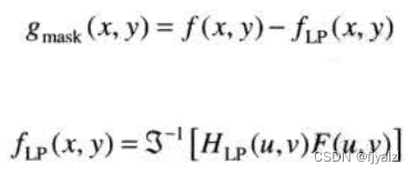
among HLP(u,v) It's a low-pass filter ,F(u,v) yes f(x,y) The Fourier transform of .fLP(x,y) Is the smoothed image .
![]()
This expression defines k=1 Passivation template and k>1 High lift filter at . We can use the frequency domain calculation involving low-pass filter or high pass filter to express the above formula
![]()
![]()
A more general formula for high-frequency emphasis filtering is :
![]()
High pass of three filters 、 Low pass code implementation :
import os

import numpy as np
import cv2
import matplotlib.pyplot as plt

plt.rcParams['font.sans-serif'] = ['SimHei']
plt.rcParams['axes.unicode_minus'] = False

#  Ideal low pass filter
def LowPassFilter(img):
    """
     Ideal low pass filter
    """
    #  The Fourier transform
    dft = cv2.dft(np.float32(img), flags=cv2.DFT_COMPLEX_OUTPUT)
    fshift = np.fft.fftshift(dft)

    #  Set the low pass filter
    rows, cols = img.shape
    crow, ccol = int(rows / 2), int(cols / 2)  #  Center position
    mask = np.zeros((rows, cols, 2), np.uint8)
    mask[crow - 20:crow + 20, ccol - 20:ccol + 20] = 1

    #  Product of mask image and spectrum image
    f = fshift * mask

    #  Inverse Fourier transform
    ishift = np.fft.ifftshift(f)
    iimg = cv2.idft(ishift)
    res = cv2.magnitude(iimg[:, :, 0], iimg[:, :, 1])
    return res


#  Ideal high pass filter
def HighPassFilter(img):
    """
     Ideal high pass filter
    """
    #  The Fourier transform
    f = np.fft.fft2(img)
    fshift = np.fft.fftshift(f)

    #  Set up the high pass filter
    rows, cols = img.shape
    crow, ccol = int(rows / 2), int(cols / 2)
    fshift[crow - 2:crow + 2, ccol - 2:ccol + 2] = 0

    #  Inverse Fourier transform
    ishift = np.fft.ifftshift(fshift)
    iimg = np.fft.ifft2(ishift)
    iimg = np.abs(iimg)
    return iimg


#  Butterworth low pass filter
def ButterworthLowPassFilter(image, d, n, s1):
    """
    Butterworth low pass filter
    """
    f = np.fft.fft2(image)
    fshift = np.fft.fftshift(f)

    def make_transform_matrix(d):
        transform_matrix = np.zeros(image.shape)
        center_point = tuple(map(lambda x: (x - 1) / 2, s1.shape))
        for i in range(transform_matrix.shape[0]):
            for j in range(transform_matrix.shape[1]):

                def cal_distance(pa, pb):
                    from math import sqrt

                    dis = sqrt((pa[0] - pb[0]) ** 2 + (pa[1] - pb[1]) ** 2)
                    return dis
                dis = cal_distance(center_point, (i, j))
                transform_matrix[i, j] = 1 / (1 + (dis / d) ** (2 * n))
        return transform_matrix


    d_matrix = make_transform_matrix(d)
    new_img = np.abs(np.fft.ifft2(np.fft.ifftshift(fshift * d_matrix)))
    return new_img


#  Butterworth high pass filter
def ButterworthHighPassFilter(image, d, n, s1):
    """
    Butterworth High pass filter
    """
    f = np.fft.fft2(image)
    fshift = np.fft.fftshift(f)

    def make_transform_matrix(d):
        transform_matrix = np.zeros(image.shape)
        center_point = tuple(map(lambda x: (x - 1) / 2, s1.shape))
        for i in range(transform_matrix.shape[0]):
            for j in range(transform_matrix.shape[1]):

                def cal_distance(pa, pb):
                    from math import sqrt

                    dis = sqrt((pa[0] - pb[0]) ** 2 + (pa[1] - pb[1]) ** 2)
                    return dis

                dis = cal_distance(center_point, (i, j))
                transform_matrix[i, j] = 1 / (1 + (d / dis) ** (2 * n))
        return transform_matrix


    d_matrix = make_transform_matrix(d)
    new_img = np.abs(np.fft.ifft2(np.fft.ifftshift(fshift * d_matrix)))
    return new_img

#  Exponential filter
def filter(img, D0, W=None, N=2, type='lp', filter='exponential'):
    '''
     Frequency domain filter
    Args:
        img:  Grayscale picture
        D0:  Cut off frequency
        W:  bandwidth
        N: butterworth And the order of the exponential filter
        type: lp, hp, bp, bs Low pass 、 qualcomm 、 Bandpass 、 Band stop
    Returns:
        imgback: The filtered image
    '''

    #  Discrete Fourier transform
    dft = cv2.dft(np.float32(img), flags=cv2.DFT_COMPLEX_OUTPUT)
    #  Centralization
    dtf_shift = np.fft.fftshift(dft)

    rows, cols = img.shape
    crow, ccol = int(rows / 2), int(cols / 2)  #  Calculate the spectrum center
    mask = np.ones((rows, cols, 2))  #  Generate rows That's ok cols Column 2 Latitude matrix
    for i in range(rows):
        for j in range(cols):
            D = np.sqrt((i - crow) ** 2 + (j - ccol) ** 2)
            if (filter.lower() == 'exponential'):  #  Exponential filter
                if (type == 'lp'):
                    mask[i, j] = np.exp(-(D / D0) ** (2 * N))
                elif (type == 'hp'):
                    mask[i, j] = np.exp(-(D0 / D) ** (2 * N))
                elif (type == 'bs'):
                    mask[i, j] = np.exp(-(D * W / (D ** 2 - D0 ** 2)) ** (2 * N))
                elif (type == 'bp'):
                    mask[i, j] = np.exp(-((D ** 2 - D0 ** 2) / D * W) ** (2 * N))
                else:
                    assert ('type error')

    fshift = dtf_shift * mask

    f_ishift = np.fft.ifftshift(fshift)
    img_back = cv2.idft(f_ishift)
    img_back = cv2.magnitude(img_back[:, :, 0], img_back[:, :, 1])  #  Calculate the absolute value of the pixel gradient
    img_back = np.abs(img_back)
    img_back = (img_back - np.amin(img_back)) / (np.amax(img_back) - np.amin(img_back))

    return img_back

def put(path):
    img = cv2.imread(path, 1)
    # img = cv2.imread(os.path.join(base, path), 1)
    img = cv2.cvtColor(img, cv2.COLOR_BGR2GRAY)
    f = np.fft.fft2(img)
    fshift = np.fft.fftshift(f)
    #  Change the complex number into a real number after taking the absolute value  #  The purpose of taking logarithm is to transform the data into 0~255
    s1 = np.log(np.abs(fshift))

    #  Display in Chinese
    plt.subplot(331)
    plt.axis('off')
    plt.title(' original image ')
    plt.imshow(img, cmap='gray')

    plt.subplot(332)
    plt.axis('off')
    plt.title(' Ideal low pass 20')
    res1 = LowPassFilter(img)
    plt.imshow(res1, cmap='gray')

    plt.subplot(333)
    plt.axis('off')
    plt.title(' Ideal high pass 2')
    res2 = HighPassFilter(img)
    plt.imshow(res2, cmap='gray')

    plt.subplot(334)
    plt.axis('off')
    plt.title(' original image ')
    plt.imshow(img, cmap='gray')

    plt.subplot(335)
    plt.axis('off')
    plt.title(' Butterworth low pass 20')
    butter_10_1 = ButterworthLowPassFilter(img, 20, 1, s1)
    plt.imshow(butter_10_1, cmap='gray')

    plt.subplot(336)
    plt.axis('off')
    plt.title(' Butterworth Qualcomm 2')
    butter_2_1_1 = ButterworthHighPassFilter(img, 2, 1, s1)
    plt.imshow(butter_2_1_1, cmap='gray')

    plt.subplot(337)
    plt.axis('off')
    plt.title(' Index the original image ')
    plt.imshow(img, cmap='gray')

    plt.subplot(338)
    plt.axis('off')
    plt.title(' Exponential low pass image 20')
    img_back = filter(img, 30, type='lp')
    plt.imshow(img_back, cmap='gray')

    plt.subplot(339)
    plt.axis('off')
    plt.title(' Exponential high pass image 2')
    img_back = filter(img, 2, type='hp')
    plt.imshow(img_back, cmap='gray')

    # plt.savefig('2.new.jpg')
    plt.show()

#  Processing function , To pass in the path
put(r'G:\4.png')

4.9 Selective filtering
The first type of filter is called band stop filter or band pass filter . The second type of filter is called notch filter .
4.9.1 Band stop filter and band pass filter
The ideal is given below 、 Expressions of Butterworth and Gaussian band stop filters , And the image form of Gaussian bandpass filter :

4.9.2 Notch filter
General form
For each filter , The distance is calculated by the following formula :

边栏推荐
猜你喜欢


随机推荐
GBASE 8C——SQL参考 5 全文检索
vim编辑器全部删除文件内容
Public opinion & spatio-temporal analysis of infectious diseases literature reading notes
2020年PHP中级面试知识点及答案
How can I get the lowest handling charge for opening a futures account?
数字图像处理 第一章 绪论
【MVC架构】MVC模型
【mysql学习】8
Minio分片上传解除分片大小限制 - chunk size must be greater than 5242880
【好文种草】根域名的知识 - 阮一峰的网络日志
How can seektiger go against the cold air in the market?
The NFT market pattern has not changed. Can okaleido set off a new round of waves?
Day 4.Social Data Sentiment Analysis: Detection of Adolescent Depression Signals
Global evidence of expressed sentimental alterations during the covid-19 pandemics
【高并发】面试官
Which futures company do you go to and how do you open an account?
mysql优化sql相关(持续补充)
Deploy redis with docker for high availability master-slave replication
How to realize master-slave synchronization in mysql5.7
Performance optimization of common ADB commands