Li Hongyi machine learning (2017 Edition)_ P6-8: gradient descent

Related information

Open source content ：https://linklearner.com/datawhale-homepage/index.html#/learn/detail/13

Open source content ：https://github.com/datawhalechina/leeml-notes

Open source content ：https://gitee.com/datawhalechina/leeml-notes

Video address ：https://www.bilibili.com/video/BV1Ht411g7Ef

Official address ：http://speech.ee.ntu.edu.tw/~tlkagk/courses.html

1、 gradient descent （Gradient Descent） Definition

Solve the minimum value of the loss function ：
$${\theta }^{\ast }=arg\min \min L(\theta )$$
$L:lossfunction（\; Loss\; function\; ）\theta :parameters（\; Parameters\; ）$
gradient descent :
Calculate the initial point respectively , Two parameters to L Partial differential of , then ${\theta }^0$ Subtract $\eta$(Learning rates（ Learning rate ）) Multiply by the value of the partial differential , Get a new set of parameters .

2、 Adjust the learning rate

2.1、 Constant learning rate problem

The learning rate is too low （ The blue line ）, The loss function drops very slowly ; Learning rate is too high （ The green line ）, The loss function drops rapidly , But soon it got stuck and didn't fall ; The learning rate is very high （ Yellow line ）, The loss function flies out ; The red one is almost just , You can get a good result .

2.2、 Adaptive learning rate （Adaptive Learning Rates）

With the increase of times , Through some factors to reduce the learning rate .
At first , The initial point will be far from the lowest point , Use a larger learning rate , Closer to the lowest point , Reduce the learning rate .
for example ：${\eta }^t=\frac{{\eta }^t}{\sqrt{t+1}}$,t It's the number of times . With the increase of times ,${\eta }^t$ Reduce .
** Be careful ：** The learning rate cannot be a value common to all characteristics , Different parameters require different learning rates

3、 Correlation optimization algorithm

3.1、Adagrad Algorithm

3.1.1、 Concept

Adagrad Algorithm means that the learning rate of each parameter divides it by the root mean square of the previous differential .

The formula is simplified as follows ：

Parameter update process ：

3.1.2、 A theoretical explanation

• For univariate function optimization ：
  

If the calculated differential is larger , The farther away from the lowest point . And the best pace is proportional to the size of the differential . So if the step is proportional to the differential , It may be better .
The greater the gradient , The farther away from the lowest point .

• For multivariable function optimization ：
  

The best iteration step is ：$\frac{A\; differential}{Quadratic\; differential}$, It is proportional to more than one differential , It's also inversely proportional to the quadratic differential .
​
about Adagrad Algorithm , The denominator $\sqrt{{\sum }_{i=0}^t(g^i{)}^2}$ Namely We hope to simulate quadratic differentiation without adding too many operations as much as possible .（ If you calculate the quadratic differential , In practice, it may increase a lot of time consumption ）.

3.2、 Random gradient descent method （Stochastic Gradient Descent）

The loss function of random gradient descent method does not need to process all the data of the training set , Instead, choose an example $x^n$ Handle （ Only one data is processed at a time ）. There is no need to process all the data as before , Just calculate the loss function of an example $Ln$, You can update the gradient .
$$L=({\hat{y}}^n-(b+\sum _i{w}_i{x}_i^n){)}^2$$$${\theta }^i={\theta }^{i-1}-n\nabla L^n({\theta }^{i-1})$$
The process comparison is as follows ：

3.3、 Feature scaling （Feature Scaling）

3.3.1、 Concept

A function has multiple input characteristics , And the distribution range of the input characteristic data is very different , It is recommended to scale their range , Make the range of different inputs the same .$$y=b+w_1{x}_1+w_2{x}_2$$

3.3.2、 reason

$x_1$ Yes y The impact of the change is relatively small , therefore $w_1$ The influence on the loss function is relatively small ,$w_1$ There is a small differential for the loss function , therefore $w_1$ It is relatively smooth in the direction , Empathy $w_2$ The direction is steep .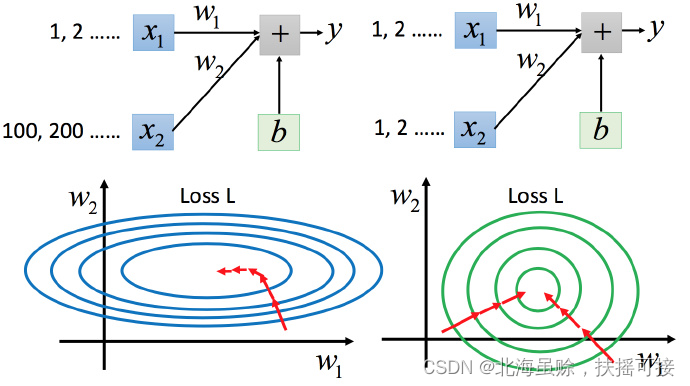

For the case on the left , As mentioned above, there is no need to Adagrad It is difficult to deal with .

• Different learning rates are required in both directions , The learning rate of the same group will not determine it . In the case on the right, it will be easier to update parameters .
• The gradient descent on the left is not towards the lowest point , But along the normal direction of the contour tangent . But green can be towards the center （ The lowest point ） go , It is also more efficient to update parameters .

3.3.3、 Zoom method

Use the batch normalization method to scale , Zoom to the standard normal distribution .

Each column above is an example , There is a set of characteristics in it .
For each dimension i（ Green box ） Calculate the average , Remember to do $m_i$; Also calculate the standard deviation , Remember to do ${\sigma }_i$.
Then use the r( features ) The... In the first example i（ data ） Inputs , Subtract the average $m_i$, Then divide by the standard deviation ${\sigma }_i$, The result is that all dimensions are 0, All variances are 1.（ Standard normal distribution ）

4、 The theoretical basis of gradient descent

4.1、 Descent visualization

stay ${\theta }^0$ It's about , The loss function can be found in a small circle ${\theta }^1$, Keep looking for .
The key is to quickly find the minimum value in the small circle .

4.2、 Taylor expansion

4.2.1、 Univariate Taylor expansion

if $h(x)$ stay $x=x_0$ There is Infinite derivative （ Infinitely differentiable ,infinitely differentiable）, So there are... In this field ：

When x Very close to $x_0$ when ,$h(x)\approx h(x_0)+h^{\prime }(x_0)(x-x_0)$.

4.2.2、 Multivariable Taylor expansion

Here is the Taylor expansion of two variables ：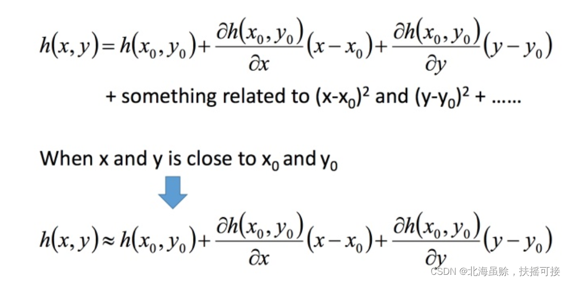

4.3、 Use Taylor expansion to solve the minimum

Taylor expansion of the loss function , At the same time, omit the infinitesimal ：

Simplified as follows ：

Use vector point multiplication , Find the minimum , Deduce GD expression ：

Be careful ： The above derivation restrictions are as follows ：
** Derivation premise ：** The estimation of the loss function given by Taylor expansion should be accurate enough , And this requires the red circle to be small enough （ That is, the learning rate is small enough ） To guarantee . So theoretically, if you want to reduce the loss function every time you update the parameters ,

4.4、 Limitation of gradient descent

It is easy to fall into local extremum It's also possible that it's not extreme , But the differential value is 0 The place of It is also possible that in practice, it stops only when the differential value is less than a certain value , But it's just gentle here , It's not the extreme point .（ It is difficult to determine the true situation ）