High level API of propeller to realize face key point detection

High level of propeller API Realize face key point detection

Project links ：https://aistudio.baidu.com/aistudio/projectdetail/1487972

One 、 Problem definition

Face key point detection , Is to input a face picture , The model will return a series of coordinates of the key points of the face , So as to locate the key information of the face .

#  Environment import 
import os
import numpy as np
import pandas as pd
import matplotlib.pyplot as plt
import matplotlib.image as mpimg

import cv2
import paddle

paddle.set_device('gpu') #  Set to GPU

import warnings 
warnings.filterwarnings('ignore') #  Ignore  warning

Two 、 Data preparation

2.1 Download datasets

The data set used in this experiment comes from github Of Open source project

At present, the data set has been uploaded to AI Studio Face key point recognition , After loading, you can directly use the following command to decompress .

!unzip data/data69065/data.zip

The structure of the decompressed data set is

data/
|—— test
|   |—— Abdel_Aziz_Al-Hakim_00.jpg
    ... ...
|—— test_frames_keypoints.csv
|—— training
|   |—— Abdullah_Gul_10.jpg
    ... ...
|—— training_frames_keypoints.csv

among ,training and test The folder stores training sets and test sets respectively .training_frames_keypoints.csv and test_frames_keypoints.csv There are labels for training sets and test sets . Next , Let's observe first training_frames_keypoints.csv file , Take a look at how the label of the training set is defined .

key_pts_frame = pd.read_csv('data/training_frames_keypoints.csv') #  Reading data sets 
print('Number of images: ', key_pts_frame.shape[0]) #  Output dataset size 
key_pts_frame.head(5) #  Look at the first five data 

    Number of images:  3462

	Unnamed: 0	0	1	2	3	4	5	6	7	8	...	126	127	128	129	130	131	132	133	134	135
0	Luis_Fonsi_21.jpg	45.0	98.0	47.0	106.0	49.0	110.0	53.0	119.0	56.0	...	83.0	119.0	90.0	117.0	83.0	119.0	81.0	122.0	77.0	122.0
1	Lincoln_Chafee_52.jpg	41.0	83.0	43.0	91.0	45.0	100.0	47.0	108.0	51.0	...	85.0	122.0	94.0	120.0	85.0	122.0	83.0	122.0	79.0	122.0
2	Valerie_Harper_30.jpg	56.0	69.0	56.0	77.0	56.0	86.0	56.0	94.0	58.0	...	79.0	105.0	86.0	108.0	77.0	105.0	75.0	105.0	73.0	105.0
3	Angelo_Reyes_22.jpg	61.0	80.0	58.0	95.0	58.0	108.0	58.0	120.0	58.0	...	98.0	136.0	107.0	139.0	95.0	139.0	91.0	139.0	85.0	136.0
4	Kristen_Breitweiser_11.jpg	58.0	94.0	58.0	104.0	60.0	113.0	62.0	121.0	67.0	...	92.0	117.0	103.0	118.0	92.0	120.0	88.0	122.0	84.0	122.0

5 rows × 137 columns

Each row in the above table represents a piece of data , among , The first column is the file name of the picture , And then from 0 Column to the first 135 Column , This is the key point information of the graph . Because each key point can be represented by two coordinates , therefore 136/2 = 68, You can see that this data set is 68 Point face key data set .

Tips1: Currently commonly used face key point annotation , Mark with the following points

• 5 spot
• 21 spot
• 68 spot
• 98 spot

Tips2： The... Used this time 68 mark , The order of marking is as follows ：

#  Calculate the mean and standard deviation of the label , Normalization for labels 
key_pts_values = key_pts_frame.values[:,1:] #  Take out the label information 
data_mean = key_pts_values.mean() #  Calculate the mean 
data_std = key_pts_values.std()   #  Calculate the standard deviation 
print(' The average value of the label is :', data_mean)
print(' The standard deviation of the label is :', data_std)

     The average value of the label is : 104.4724870017331
     The standard deviation of the label is : 43.17302271754281

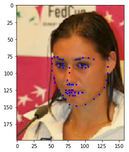
2.2 Look at the image

def show_keypoints(image, key_pts):    """ Args: image:  Image information  key_pts:  Key point information ,  Show pictures and key information  """    plt.imshow(image.astype('uint8'))  #  Show picture information  for i in range(len(key_pts)//2,): plt.scatter(key_pts[i*2], key_pts[i*2+1], s=20, marker='.', c='b') #  Show key information 

#  Display a single piece of data 

n = 14 # n Index data in a table  
image_name = key_pts_frame.iloc[n, 0] #  Get image name 
key_pts = key_pts_frame.iloc[n, 1:].values #  The image label Format to numpy.array The format of 
key_pts = key_pts.astype('float').reshape(-1) #  Get image key information 
print(key_pts.shape)
plt.figure(figsize=(5, 5)) #  The size of the displayed image 
show_keypoints(mpimg.imread(os.path.join('data/training/', image_name)), key_pts) #  Display images and key point information 
plt.show() #  Show the image 

    (136,)

2.3 Dataset definition

Use the propeller frame API Of paddle.io.Dataset Custom dataset class , Please refer to the official website for details Custom datasets .

according to __init__ Defined in the , Realization __getitem__ and __len__.

#  according to Dataset The standard of use , Build face key point data set 

from paddle.io import Dataset

class FacialKeypointsDataset(Dataset):
    #  Face key data set 
    """  Step one ： Inherit paddle.io.Dataset class  """
    def __init__(self, csv_file, root_dir, transform=None):
        """  Step two ： Implement constructors , Define the dataset size  Args: csv_file (string):  Marked csv File path  root_dir (string):  Folder path of image storage  transform (callable, optional):  Data processing method applied to image  """
        self.key_pts_frame = pd.read_csv(csv_file) #  Read csv file 
        self.root_dir = root_dir #  Get the picture folder path 
        self.transform = transform #  obtain  transform  Method 

    def __getitem__(self, idx):
        """  Step three ： Realization __getitem__ Method , The definition specifies index How to get data when , And return a single piece of data （ Training data , Corresponding label ） """

        image_name = os.path.join(self.root_dir,self.key_pts_frame.iloc[idx,0])

        #  Get images 
        image = mpimg.imread(image_name)

        #  Image format processing , If you include alpha passageway , Then ignore him , Only take the first three channels 
        if(image.shape[2] == 4):
            image = image[:,:,0:3]

        #  Get key information 
        key_pts = self.key_pts_frame.iloc[idx,1:].values
        key_pts = key_pts.astype('float').reshape(-1) # [136,1]

        #  If you define transform Method , Use transform Method 
        if self.transform:
            image,key_pts = self.transform([image,key_pts])
        
        #  To numpy Data format 
        image = np.array(image,dtype='float32')
        key_pts = np.array(key_pts,dtype='float32')

        return image, key_pts

    def __len__(self):
        """  Step four ： Realization __len__ Method , Returns the total number of datasets  """
        return len(self.key_pts_frame) #  Return dataset size , That is, the number of pictures 

2.4 Training set visualization

Instantiate the dataset and display some images .

#  Build a dataset class 
face_dataset = FacialKeypointsDataset(csv_file='data/training_frames_keypoints.csv',
                                      root_dir='data/training/')

#  Output dataset size 
print(' The data set size is : ', len(face_dataset))
#  according to  face_dataset  Visual datasets 
num_to_display = 3

for i in range(num_to_display):
    
    #  Define image size 
    fig = plt.figure(figsize=(20,10))
    
    #  Randomly select pictures 
    rand_i = np.random.randint(0, len(face_dataset))
    sample = face_dataset[rand_i]

    #  Output picture size and number of keys 
    print(i, sample[0].shape, sample[1].shape)

    #  Set picture printing information 
    ax = plt.subplot(1, num_to_display, i + 1)
    ax.set_title('Sample #{}'.format(i))
    
    #  Output pictures 
    show_keypoints(sample[0], sample[1])

     The data set size is :  34620 (211, 186, 3) (136,)1 (268, 228, 3) (136,)2 (191, 164, 3) (136,)

Although the above code completes the definition of the data set , But there are still some problems , Such as ：

• The size of each image is different , The image size needs to be unified to meet the network input requirements
• The image format needs to adapt to the format input requirements of the model
• The amount of data is relatively small , No data enhancement

These problems will affect the final performance of the model , So we need to preprocess the data .

2.5 Transforms

Preprocess the image , Including graying 、 normalization 、 Resize 、 Random cutting , Modify the channel format and so on , To meet the data requirements ; The functions of each category are as follows ：

• Graying ： Discard color information , Preserve image edge information ; The recognition algorithm is not strongly dependent on color , The robustness will decrease after adding color , And the dimension of grayscale image decreases （3->1）, Keeping the gradient will speed up the calculation .
• normalization ： Speed up convergence
• Resize ： Data to enhance
• Random cutting ： Data to enhance
• Modify the channel format ： Change to the structure required by the model

#  Standardized customization  transform  Method 

class TransformAPI(object):
    """  Step one ： Inherit  object  class  """
    def __call__(self, data):

        """  Step two ： stay  __call__  Define data processing methods in  """
        
        processed_data = data
        return  processed_data

import paddle.vision.transforms.functional as F

class GrayNormalize(object):
    #  Change the picture to grayscale , And reduce its value to [0, 1]
    #  take  label  Zoom in to  [-1, 1]  Between 

    def __call__(self, data):
        image = data[0]   #  Get photo 
        key_pts = data[1] #  Get tag 
        
        image_copy = np.copy(image)
        key_pts_copy = np.copy(key_pts)

        #  Grayscale the picture 
        gray_scale = paddle.vision.transforms.Grayscale(num_output_channels=3)
        image_copy = gray_scale(image_copy)
        
        #  Zoom the picture value to  [0, 1]
        image_copy = image_copy / 255.0
        
        #  Zoom the coordinate point to  [-1, 1]
        mean = data_mean #  Get the average value of the tag 
        std = data_std   #  Get the standard deviation of the label 
        key_pts_copy = (key_pts_copy - mean)/std

        return image_copy, key_pts_copy

class Resize(object):
    #  Adjust the input image to the specified size 

    def __init__(self, output_size):
        assert isinstance(output_size, (int, tuple))
        self.output_size = output_size

    def __call__(self, data):

        image = data[0]    #  Get photo 
        key_pts = data[1]  #  Get tag 

        image_copy = np.copy(image)      
        key_pts_copy = np.copy(key_pts)

        h, w = image_copy.shape[:2]
        if isinstance(self.output_size, int):
            if h > w:
                new_h, new_w = self.output_size * h / w, self.output_size
            else:
                new_h, new_w = self.output_size, self.output_size * w / h
        else:
            new_h, new_w = self.output_size

        new_h, new_w = int(new_h), int(new_w)

        img = F.resize(image_copy, (new_h, new_w))
        
        # scale the pts, too
        key_pts_copy[::2] = key_pts_copy[::2] * new_w / w
        key_pts_copy[1::2] = key_pts_copy[1::2] * new_h / h

        return img, key_pts_copy


class RandomCrop(object):
    #  Crop the input image at random position 

    def __init__(self, output_size):
        assert isinstance(output_size, (int, tuple))
        if isinstance(output_size, int):
            self.output_size = (output_size, output_size)
        else:
            assert len(output_size) == 2
            self.output_size = output_size

    def __call__(self, data):
        image = data[0]
        key_pts = data[1]

        image_copy = np.copy(image)
        key_pts_copy = np.copy(key_pts)

        h, w = image_copy.shape[:2]
        new_h, new_w = self.output_size

        top = np.random.randint(0, h - new_h)
        left = np.random.randint(0, w - new_w)

        image_copy = image_copy[top: top + new_h,
                      left: left + new_w]

        key_pts_copy[::2] = key_pts_copy[::2] - left
        key_pts_copy[1::2] = key_pts_copy[1::2] - top

        return image_copy, key_pts_copy

class ToCHW(object):
    #  Change the format of the image from HWC Change it to CHW
    def __call__(self, data):
        
        image = data[0]
        key_pts = data[1]

        transpose = T.Transpose((2,0,1))
        image = transpose(image)
        
        return image, key_pts

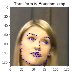
Take a look at the effect of each image preprocessing method .

import paddle.vision.transforms as T

#  test  Resize
resize = Resize(256)

#  test  RandomCrop
random_crop = RandomCrop(128)

#  test  GrayNormalize
norm = GrayNormalize()

#  test  Resize + RandomCrop, The image size changes to 250*250,  Then cut out 224*224 The image block of 
composed = paddle.vision.transforms.Compose([Resize(250), RandomCrop(224)])

test_num = 800 #  Test data subscript 
data = face_dataset[test_num]

transforms = {
    'None': None, 
              'norm': norm,
              'random_crop': random_crop,
              'resize': resize ,
              'composed': composed}
for i, func_name in enumerate(['None', 'norm', 'random_crop', 'resize', 'composed']):
    
    #  Define image size 
    fig = plt.figure(figsize=(20,10))
    
    #  Processing images 
    if transforms[func_name] != None:
        transformed_sample = transforms[func_name](data)
    else:
        transformed_sample = data

    #  Set picture printing information 
    ax = plt.subplot(1, 5, i + 1)
    ax.set_title(' Transform is #{}'.format(func_name))
    
    #  Output pictures 
    show_keypoints(transformed_sample[0], transformed_sample[1])

2.6 Use data preprocessing to complete data definition

Let's go Resize、RandomCrop、GrayNormalize、ToCHW Apply to new data sets

from paddle.vision.transforms import Compose

data_transform = Compose([Resize(256), RandomCrop(224), GrayNormalize(), ToCHW()])

# create the transformed dataset
train_dataset = FacialKeypointsDataset(csv_file='data/training_frames_keypoints.csv',
                                       root_dir='data/training/',
                                       transform=data_transform)
print('Number of train dataset images: ', len(train_dataset))

for i in range(4):
    sample = train_dataset[i]
    print(i, sample[0].shape, sample[1].shape)

test_dataset = FacialKeypointsDataset(csv_file='data/test_frames_keypoints.csv',
                                             root_dir='data/test/',
                                             transform=data_transform)

print('Number of test dataset images: ', len(test_dataset))

Number of train dataset images:  3462
0 (3, 224, 224) (136,)
1 (3, 224, 224) (136,)
2 (3, 224, 224) (136,)
3 (3, 224, 224) (136,)
Number of test dataset images:  770

3、 Model building

3.1 Networking can be very simple

According to the above analysis, we can see , Face key point detection and classification , The same network structure can be used , Such as LeNet、Resnet50 When the feature extraction is completed , Just on the original basis , The last part of the model needs to be modified , Adjust the output to Number of face keys *2, That is, the abscissa and ordinate of each face key point , You can complete the task of face key point detection , See the following code for details , You can also refer to the case on the official website : Face key point detection

The network structure is as follows ：

import paddle.nn as nn
from paddle.vision.models import resnet50
class SimpleNet(nn.Layer):
    
    def __init__(self, key_pts):

        super(SimpleNet, self).__init__()

        #  Use resnet50 As backbone
        self.backbone = paddle.vision.models.resnet50(pretrained= True)

        #  Add the first linear transformation layer 
        self.linear1 = nn.Linear(in_features=1000, out_features= 512)

        #  Use ReLU Activation function 
        self.act1 = nn.ReLU()

        #  Add a second linear transformation layer as the output , The number of output elements is  key_pts*2, Coordinates representing each key point 
        self.linear2 = nn.Linear(in_features= 512,out_features= key_pts*2)

    def forward(self, x):

        x = self.backbone(x)
        x = self.linear1(x)
        x = self.act1(x)
        x = self.linear2(x)

        return x

3.2 Network structure visualization

Use model.summary Visual network structure .

model = paddle.Model(SimpleNet(key_pts=68))
# random_crop [224, 224, 3]
# to_chw [3, 224, 224]
model.summary((-1, 3, 224, 224))

Four 、 model training

4.1 The model configuration

Before training the model , You need to set the optimizer required by the training model , Loss function and evaluation index .

• Optimizer ：Adam Optimizer , Fast convergence .
• Loss function ：SmoothL1Loss
• Evaluation indicators ：NME

4.2 Custom evaluation indicators

Task specific Metric The calculation method is existing in the frame Metric There is no... In the interface , Or the algorithm does not meet their own needs , Then we need to do it ourselves Metric The custom of . Here's how to Metric Custom operation of , For more information, please refer to the official website Customize Metric; Let's start with the following code .

from paddle.metric import Metric

class NME(Metric):
    """ 1.  Inherit paddle.metric.Metric """
    def __init__(self, name='nme', *args, **kwargs):
        """ 2.  Constructor implementation , Just customize the parameters  """
        super(NME, self).__init__(*args, **kwargs)
        self._name = name
        self.rmse = 0
        self.sample_num = 0
    
    def name(self):
        """ 3.  Realization name Method , Return the defined evaluation indicator name  """
        return self._name
    
    def update(self, preds, labels):
        """ 4.  Realization update Method , For a single batch Calculate the evaluation index during training . -  When `compute` When a class function is not implemented , The calculated output of the model and the flattening of the label data will be used as `update` Parameters passed in . """
        N = preds.shape[0]

        preds = preds.reshape((N, -1, 2))
        labels = labels.reshape((N, -1, 2))

        self.rmse = 0
        
        for i in range(N):
            pts_pred, pts_gt = preds[i, ], labels[i, ]
            interocular = np.linalg.norm(pts_gt[36, ] - pts_gt[45, ])

            self.rmse += np.sum(np.linalg.norm(pts_pred - pts_gt, axis=1)) / (interocular * preds.shape[1])
            self.sample_num += 1

        return self.rmse / N
    
    def accumulate(self):
        """ 5.  Realization accumulate Method , Back to history batch The evaluation index value calculated after training accumulation .  Every time `update` Data accumulation during call ,`accumulate` During calculation, all accumulated data are calculated and returned .  The settlement result will be in `fit` In the training log of the interface . """
        return self.rmse / self.sample_num
    
    def reset(self):
        """ 6.  Realization reset Method , Every Epoch Reset the evaluation index after completion , So next Epoch You can recalculate . """
        self.rmse = 0
        self.sample_num = 0

4.3 Realize the configuration and training of the model

#  Use  paddle.Model  Packaging model 
model = paddle.Model(SimpleNet(key_pts=68))

#  Definition Adam Optimizer 
optimizer = paddle.optimizer.Adam(learning_rate=0.001,weight_decay=5e-4,parameters=model.parameters())

#  Definition SmoothL1Loss
loss = nn.SmoothL1Loss()

#  Use customization metrics
metric = NME()

#  Configuration model 
model.prepare(optimizer = optimizer, loss=loss, metrics = metric)

The choice of loss function ：L1Loss、L2Loss、SmoothL1Loss Comparison of

• L1Loss: At the end of training , Forecast value and ground-truth The difference is small , The absolute value of the derivative of the loss to the predicted value is still 1, At this time, if the learning rate remains unchanged , The loss function will fluctuate near the stable value , It is difficult to continue to converge to higher accuracy .
• L2Loss: At the beginning of training , Forecast value and ground-truth When the difference is large , The gradient of the loss function to the predicted value is very large , Lead to unstable training .
• SmoothL1Loss: stay x More hours , Yes x The gradient will also decrease , And in the x When a large , Yes x The absolute value of the gradient reaches the upper limit 1, It's not too big to break the network parameters .

 model.fit(train_dataset,epochs=50, batch_size=64,verbose =1)

4.4 Model preservation

checkpoints_path = './checkpoints/models'
model.save(checkpoints_path)

5、 ... and 、 Model to predict

#  Define function 

def show_all_keypoints(image, predicted_key_pts):
    """  Show the image , Predict the key points  Args： image： Cropped image  [224, 224, 3] predicted_key_pts:  Coordinates of key points of prediction  """
    #  Show the image 
    plt.imshow(image.astype('uint8'))

    #  Show key points 
    for i in range(0, len(predicted_key_pts), 2):
        plt.scatter(predicted_key_pts[i], predicted_key_pts[i+1], s=20, marker='.', c='m')

def visualize_output(test_images, test_outputs, batch_size=1, h=20, w=10):
    """  Show the image , Predict the key points  Args： test_images： Cropped image  [224, 224, 3] test_outputs:  Model output  batch_size:  Batch size  h:  The displayed image is high  w:  The displayed image is wide  """

    if len(test_images.shape) == 3:
        test_images = np.array([test_images])

    for i in range(batch_size):

        plt.figure(figsize=(h, w))
        ax = plt.subplot(1, batch_size, i+1)

        #  Randomly cropped image 
        image = test_images[i]

        #  Model output , Unreduced predicted key coordinate values 
        predicted_key_pts = test_outputs[i]

        #  Restore the real key coordinate value 
        predicted_key_pts = predicted_key_pts * data_std + data_mean
        
        #  Show images and key points 
        show_all_keypoints(np.squeeze(image), predicted_key_pts)
            
        plt.axis('off')

    plt.show()

#  Read images 
img = mpimg.imread('xiaojiejie.jpg')

#  Key placeholder 
kpt = np.ones((136, 1))

transform = Compose([Resize(256), RandomCrop(224)])

#  Redefine the size of the image first , And cut it to  224*224 Size 
rgb_img, kpt = transform([img, kpt])

norm = GrayNormalize()
to_chw = ToCHW()

#  Normalize and format transform the image 
img, kpt = norm([rgb_img, kpt])
img, kpt = to_chw([img, kpt])

img = np.array([img], dtype='float32')

#  Load the saved model for prediction 
model = paddle.Model(SimpleNet(key_pts=68))
model.load(checkpoints_path)
model.prepare()

#  Predicted results 
out = model.predict_batch([img])
out = out[0].reshape((out[0].shape[0], 136, -1))

#  visualization 
visualize_output(rgb_img, out, batch_size=1)

6、 ... and 、 Interesting application

When we get the key information , You can make some interesting applications .

#  Define function 

def show_fu(image, predicted_key_pts):
    """  Show the pasted image  Args： image： Cropped image  [224, 224, 3] predicted_key_pts:  Coordinates of key points of prediction  """
    #  Calculate the coordinate ,15  and  34 The middle value of the point 
    x = (int(predicted_key_pts[28]) + int(predicted_key_pts[66]))//2
    y = (int(predicted_key_pts[29]) + int(predicted_key_pts[67]))//2

    #  open   Little picture of Spring Festival 
    star_image = mpimg.imread('light.jpg')

    #  Processing channels 
    if(star_image.shape[2] == 4):
        star_image = star_image[:,:,1:4]
    
    #  Put the small picture of Spring Festival on the original picture 
    image[y:y+len(star_image[0]), x:x+len(star_image[1]),:] = star_image
    
    #  Show the processed picture 
    plt.imshow(image.astype('uint8'))

    #  Show key information 
    for i in range(len(predicted_key_pts)//2,):
        plt.scatter(predicted_key_pts[i*2], predicted_key_pts[i*2+1], s=20, marker='.', c='m') #  Show key information 


def custom_output(test_images, test_outputs, batch_size=1, h=20, w=10):
    """  Show the image , Predict the key points  Args： test_images： Cropped image  [224, 224, 3] test_outputs:  Model output  batch_size:  Batch size  h:  The displayed image is high  w:  The displayed image is wide  """

    if len(test_images.shape) == 3:
        test_images = np.array([test_images])

    for i in range(batch_size):

        plt.figure(figsize=(h, w))
        ax = plt.subplot(1, batch_size, i+1)

        #  Randomly cropped image 
        image = test_images[i]

        #  Model output , Unreduced predicted key coordinate values 
        predicted_key_pts = test_outputs[i]

        #  Restore the real key coordinate value 
        predicted_key_pts = predicted_key_pts * data_std + data_mean
        
        #  Show images and key points 
        show_fu(np.squeeze(image), predicted_key_pts)
            
        plt.axis('off')

    plt.show()

#  Read images 
img = mpimg.imread('xiaojiejie.jpg')

#  Key placeholder 
kpt = np.ones((136, 1))

transform = Compose([Resize(256), RandomCrop(224)])

#  Redefine the size of the image first , And cut it to  224*224 Size 
rgb_img, kpt = transform([img, kpt])

norm = GrayNormalize()
to_chw = ToCHW()

#  Normalize and format transform the image 
img, kpt = norm([rgb_img, kpt])
img, kpt = to_chw([img, kpt])

img = np.array([img], dtype='float32')

#  Load the saved model for prediction 
# model = paddle.Model(SimpleNet())
# model.load(checkpoints_path)
# model.prepare()

#  Predicted results 
out = model.predict_batch([img])
out = out[0].reshape((out[0].shape[0], 136, -1))

#  visualization 
custom_output(rgb_img, out, batch_size=1)