Self learning neural network series - 8 feedforward neural networks

What you need to know before reading this article is shown in Feedforward neural network pre knowledge This article , It mainly includes perceptron algorithm 、 Activation function and other knowledge , The following mainly introduces the content of feedforward neural network , There are mainly ：

• 8.1 Feedforward neural network structure
• 8.2 Learning of neural network parameters
• 8.3 Error back propagation algorithm
• 8.4 tensorflow The principle of automatic gradient calculation in
• 8.5 How to solve Nonconvex Optimization in machine learning or deep learning

1 Feedforward neural network structure

1.1 Network structure

• Feedforward neural network is a generalized structure of neural network model , All neurons are connected , Also known as fully connected neural network , The structure is as follows ： By an input layer 、 Multiple hidden layers and one output layer constitute .
  

chart 1 All connected neural networks （《 Neural networks and deep learning 》( Qiu Xipeng )）

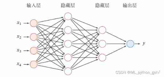
• The layers in the neural network are composed of multiple neurons
  • Input layer neurons have numerical characteristics such as x = (x1,x2,x3,x4) constitute ,
  • Hidden layer neurons are activation functions
  • Output layer neurons are linear functions （ Return to ）、sigmoid function （ Two classification ） or softmax function （ Many classification ）
  • Connections between neurons （ edge ） For weight , Point to the edges of the same neuron for linear combination , And then output through neurons .

1.2 A network model

• The feedforward neural network model is propagated forward by the following formula ：
  $$\{\begin{array}{l}{z}^i=W^i{a}^{i-1}+b^i\\ a^i=sigmoid(z^i)\end{array}$$

• $Make{a}^0=x$, By the end of i The layer is the perspective , For any two connected neurons :

  • Previous hidden layer output / Input layer input ：$a^{i-1}$
  • Hidden layer input / Input layer output ：$z^i=W^i{a}^{i-1}+b^i$
  • Hidden layer output ：$a^i=sigmoid(z^i)$
  • Iterate until the model structure is satisfied

• General approximation theorem ： Common continuous nonlinear functions can be approximated by feedforward neural networks .

• Deep learning is mainly based on neural network model , The neural network model can be regarded as a complex high-order nonlinear function .

• Machine learning is based on simple models , Artificial feature engineering is very important , Play a decisive role in the model . However , Manual features require time-consuming design and verification , And it is easy to cause information loss , Therefore, neural network is introduced to automatically learn the expression of features .

2 Learning parameters of feedforward neural network

• Parameter learning method ： Similar to machine learning , The learning of neural network parameters is also aimed at minimizing the loss function , The optimization method uses the common gradient descent .

2.1 Objective function

$$\begin{gathered} R(W,b)=\frac{1}{N}\sum _{n=1}^{N}L(y^n,{\hat{y}}^n)+\lambda ||W|{|}_F^2 \\ Itsin||W|{|}_F^2=\sum _l^L\sum _i^{M_l}\sum _j^{M_{l-1}}{w}_{ij}^2 \end{gathered}$$

2.2 gradient descent

• Final output $\hat{y}$ And y The loss function is constructed for $l$ Layer parameters ( to update )$W^l、b^l$ Finding the gradient has ：
  $$\begin{gathered} \frac{\partial R(W,b)}{\partial W^l}=\frac{1}{N}\sum _{n=1}^N\frac{\partial L(y^n,{\hat{y}}^n)}{\partial W^l}+\lambda W^l \\ \frac{\partial R(W,b)}{\partial b^l}=\frac{1}{N}\sum _{n=1}^N\frac{\partial L(y^n,{\hat{y}}^n)}{\partial b^l} \end{gathered}$$
• The whole training set is needed to solve the parameters of each layer , Neural networks usually use the random gradient descent method to update the parameters of a single sample or min-batch The gradient descent method is used to update the parameters of batch samples .
• It is inefficient to update parameters by calculating the gradient expression of parameters , Neural networks usually use error back propagation algorithm to achieve efficient gradient calculation .

3 Error back propagation algorithm

• The chain rule ：

$$\begin{gathered} \frac{\partial L(y^n,{\hat{y}}^n)}{\partial W_{ij}^l}=\frac{\partial L(y^n,{\hat{y}}^n)}{\partial z^l}\frac{\partial z^l}{\partial W_{ij}^l} \\ \frac{\partial L(y^n,{\hat{y}}^n)}{\partial b^l}=\frac{\partial L(y^n,{\hat{y}}^n)}{\partial z^l}\frac{\partial z^l}{\partial b^l} \end{gathered}$$

• Factor analysis

  • $\frac{\partial L(y^n,{\hat{y}}^n)}{\partial z^l}$ Is a duplicate , So we only need to calculate three terms ：

  • $\frac{\partial L(y^n,{\hat{y}}^n)}{\partial z^l}$ Is the loss function for the $l$ The derivative of the linear combination of layers , Finally, it is conducted through neurons , It reflects the second stage $l$ The influence of layer and its subsequent neurons on the loss function , The inclusion of a loss function is called an error term .

  • $\frac{\partial z^l}{\partial W_{ij}^l}、\frac{\partial z^l}{\partial b^l}$ Similar to perceptron algorithm , The gradient method is similar to .

  • The main difficulty is to solve the error term ： Back propagation algorithm

• Error back propagation iteration formula

$$\delta (l)=\frac{\partial L(y^n,{\hat{y}}^n)}{\partial z^l}=\frac{\partial L(y^n,{\hat{y}}^n)}{\partial z^{l+1}}\frac{\partial z^{l+1}}{\partial a^l}\frac{\partial a^l}{\partial z^l}=\delta (l+1)W^{l+1}sigmoi{d}^{\prime }(z^l)$$

• The error term can be solved iteratively , The other items are easy to calculate

• Error back propagation algorithm

  • Feedforward calculates the linear output of each layer $z^l$ And nonlinear output $a^l$
  • For the last layer, the error term is calculated as a single-layer perceptron （ Easy to calculate ）、 gradient 、 Update parameters
  • Next, the error term of each layer is calculated according to the iterative formula
  • Calculate the gradient of each layer of perceptron and update the parameters

4 tensorflow The principle of automatic gradient calculation in

• Calculation chart ：tensorflow In this paper, the automatic calculation of gradient is realized by using the data structure such as calculation graph
• Basic concept of calculation diagram ：
  

chart 2 Calculation chart （《 Neural networks and deep learning 》( Qiu Xipeng )）

• The calculation diagram decomposes the complex calculation process , Use intermediate nodes to represent the operation , Place the intermediate calculation result on the arrow of the node （ edge ） On , Other nodes pointing to the middle node represent constants or variables .

  • The calculation chart supports local calculation , The intermediate result is calculated , So in the process of calculating the derivative, we can keep the intermediate result , Calculate the local derivative , Then pass it to the next layer
  • From left to right, the calculation diagram shows the forward propagation formula of neural network , So we can see the error back propagation from the calculation diagram , That is, the calculation diagram is viewed from right to left .
  • The local derivative of the addition in the calculation graph is 1; The local derivative of multiplication is another factor ;

• The forward model uses the chain rule to calculate the intermediate result of the gradient W For each dimension of , The intermediate process of using chain rule to calculate gradient in reverse mode only involves Z For each dimension of . Therefore, when the output dimension is much smaller than the input dimension, the back propagation algorithm should be used .

• tensorflow The calculation diagram is divided into static calculation diagram 、 Dynamic calculation diagram and Autograph

  • Static calculation diagram ： First use TensorFlow Definition of various operators to create a complete calculation diagram , And then open a conversation Session, Perform the calculation diagram explicitly . Once defined , It can't be changed any more .
  • Dynamic calculation diagram ： Every time you use an operator , This operator will be automatically added to the default calculation diagram , No need to start session, Directly execute to get the result . Convenient debugging , You can change .
  • Autograph： have access to @tf.function Decorators will be defined Python Function is converted to the corresponding TensorFlow Static calculation diagram construction code .

5 Nonconvex Optimization in deep learning

• Loss functions in deep learning are generally non convex , Why is the loss function of neural network non convex ?
• Nonconvex Optimization
  • The objective function is not convex
  • Feasible sets are not convex sets :Lasso\ Sparse matrix factorization belongs to this class
  • A large number of local optimal solutions , The local optimal solution is not necessarily the global optimal solution
  • Generally, gradient descent method is used to solve
• Non convex optimization solution ideas
  • Convex relaxation ： Lagrange duality method to modify the objective function （ Convex function ） And constraints （ convex set ）
  • Gradient descent of nonconvex projection ：Lasso/ Recommend matrix decomposition in the system , Project a sparse matrix onto a low rank matrix , Rank conditions form Nonconvex Sets . gradient descent 、 Projection update 、 gradient descent 、 Projection update …
  • Alternate optimization ： stay ALS In the algorithm, , Although the objective function is non convex , But it may be a convex function in a certain component direction
  • EM Algorithm etc.
  • The algorithm can be referred to ：Non-convex Optimization for Machine Learning
• Neural network optimization problem
  • There are many saddle points in high dimension , It is not easy to fall into local optimization
  • In order to ensure generalization ability , Prevent over fitting , It is not necessary to solve the global minimum