Meta agent model can be migrated to resist attacks

1 introduction

  This paper is about the portability of black box attacks . In the current large number of studies , Many methods directly attack the agent model and obtain the transferable countermeasure samples to deceive the target model , However, due to the mismatch between the agent model and the target model , Their attack effects are limited . In this paper , The author solves this problem from a new angle , By training a meta agent model （MSM）, So that attacks on this model can be more easily migrated to other models . The objective function of this method is mathematically expressed as a two-level optimization problem , In order to make the training process gradient effective , A new gradient updating process is proposed , It is proved theoretically that . Experimental results show that , By attacking meta agent model , We can obtain more transportable countermeasure samples to cheat the black box model including countermeasure training , The attack success rate is much higher than the existing methods . According to the algorithm framework , I use pytorch A simple code implementation , Interested people can change the data set part of the code and try to run .
Thesis link ： https://arxiv.org/abs/2109.01983

2 Preliminary knowledge

  FGSM Attack is a single step attack based on gradient , The classification loss function is increased by using the gradient rising method , Thus, the classification confidence of the target classifier is reduced . The formula is as follows ：$$x_{adv}=\mathrm{C}\mathrm{l}\mathrm{i}\mathrm{p}(x+ϵ\cdot \mathrm{s}\mathrm{i}\mathrm{g}\mathrm{n}({\nabla }_{x}L(f(x),y)))$$ among $x$ It is a clean sample ,$x_{adv}$ To counter the sample ,$y$ Is the corresponding category label ,$ϵ$ Is the attack step size , And there are $ϵ<L_{\infty }$.$f$ Is the target classifier being attacked ,$\mathrm{C}\mathrm{l}\mathrm{i}\mathrm{p}$ Is a truncation function ,$L$ Is the cross entropy loss function .
 PGD An attack is an extension FGSM Multi step attack mode of attack , The specific formula is as follows ：$$x_{adv}^k=\mathrm{C}\mathrm{l}\mathrm{i}\mathrm{p}(x_{adv}^{k-1}+\frac{ϵ}{T}\cdot \mathrm{s}\mathrm{i}\mathrm{g}\mathrm{n}({\nabla }_{x_{adv}^{k-1}}L(f(x_{adv}^{k-1}),y)))$$$x_{adv}^k$ For the first time $k$ Counter samples generated in step , also $x_{adv}^0$ Indicates the initial clean sample , The number of iterations of the attack is $T$.

3 Paper method

  For black box attacks , The internal parameter information of the target model is hidden from the attacker and query access is not allowed . Attackers can only access data sets used by the target model , And a single or group of source models that share a dataset with the target model . The existing transportable anti attack methods carry out various attacks on these source models , And hope to obtain the transferable countermeasure samples that can deceive the unknown target model . In this paper, the author proposes a new meta learning migration attack framework to train meta agent model , Its goal is to attack the meta agent model to produce more powerful transferable countermeasures than the original model .
  Make $\mathcal{A}$ To counter attack algorithms ,${\mathcal{M}}_{\theta }$ Is with a parameter of $\theta$ Meta - agent model , Give a sample $x$, attack ${\mathcal{M}}_{\theta }$ The counter sample of can be expressed as $$\mathcal{A}({\mathcal{M}}_{\theta },x,y)=x_{adv}=\mathrm{C}\mathrm{l}\mathrm{i}\mathrm{p}(x+ϵ\cdot \mathrm{s}\mathrm{i}\mathrm{g}\mathrm{n}({\nabla }_{x}L({\mathcal{M}}_{\theta }(x),y)))$$ Because when attacking , Only one set of source models can be obtained ${\mathcal{F}}_1,\cdots ,{\mathcal{F}}_N$, So we need to evaluate the countermeasure samples in the source model $\mathcal{A}({\mathcal{M}}_{\theta },x,y)$ The portability of , And by maximizing this $N$ The meta agent model is optimized by using the parameters of the source model , The specific form is as follows $$\arg \underset{\theta }{\max }{\mathbb{E}}_{(x,y)\sim D}\left[\sum _{i=1}^{N}L({\mathcal{F}}_i(\mathcal{A}({\mathcal{M}}_{\theta },x,y)),y)\right]$$ among $D$ For the distribution of training data . The structure and training process of the goal are shown in the figure below , It can be regarded as a meta learning or two-level optimization method . In Inner optimization , The counter sample is generated by the white box attack on the meta proxy model, which is usually a gradient rising method , And in outer optimization , The authors send the countermeasure samples into the source model to calculate the robust loss .

• In the process of generating countermeasure samples by inner layer optimization , The author designed a self-made PGD Attack methods , The original PGD Attack because of $\mathrm{s}\mathrm{i}\mathrm{g}\mathrm{n}$ function , The gradient will disappear when the network parameters are updated for back propagation . Is the first $k$ Step generated gradient $g_{ens}^k$ The calculation formula of is as follows ：$$\{\begin{array}{rl}{g}_1^k& =\frac{g^k}{\mathrm{s}\mathrm{u}\mathrm{m}(\mathrm{a}\mathrm{b}\mathrm{s}(g^k))}\\ g_t^k& =\frac{2}{\pi }\cdot \mathrm{a}\mathrm{r}\mathrm{c}\mathrm{t}\mathrm{a}\mathrm{n}(\frac{g^k}{\mathrm{m}\mathrm{e}\mathrm{a}\mathrm{n}(\mathrm{a}\mathrm{b}\mathrm{s}(g^k))})\\ g_s^k& =\mathrm{s}\mathrm{i}\mathrm{g}\mathrm{n}(g^k)\\ g_{ens}^k& =g_1^k+{\gamma }_1\cdot g_t^k+{\gamma }_2\cdot g_s^k\end{array}$$ Make ${\gamma }_1={\gamma }_2=0.01$,$g_1^k$ and $g_2^k$ Ensure that the objective function is differentiable with respect to the parameters of the meta surrogate model ,$\mathrm{a}\mathrm{r}\mathrm{c}\mathrm{t}\mathrm{a}\mathrm{n}$ Is an approximation of a symbolic function ,$\frac{1}{\mathrm{m}\mathrm{e}\mathrm{a}\mathrm{n}(\mathrm{a}\mathrm{b}\mathrm{s}(g^k))}$ prevent $\mathrm{a}\mathrm{r}\mathrm{c}\mathrm{t}\mathrm{a}\mathrm{n}$ Fall into a linear region .${\gamma }_2\cdot g_s^k$ by $g_{ens}^k$ Each pixel of provides a lower bound . The formula for generating countermeasure samples is as follows ：$$x_{adv}^k=\mathrm{C}\mathrm{l}\mathrm{i}\mathrm{p}(x_{adv}^{k-1}+\frac{{ϵ}_c}{T}\cdot g_{ens}^{k-1})$$ iteration $T$ Get the final confrontation sample after step $x_{adv}^T$.
• Countermeasure samples to be generated $x_{adv}^T$ Input to $N$ Calculate the corresponding countermeasure loss in the three meta models $L({\mathcal{F}}_i(x_{adv}^T),y)$,$N$ The greater the confrontation loss of the source model, the greater the generated confrontation samples generated by the agent model $x_{adv}^T$ There is also a higher possibility to cheat the source model .
• The weight parameters of the network are optimized by maximizing the objective function of the meta agent model , The specific parameter optimization formula is as follows $${\theta }^{\prime }=\theta +\alpha \cdot \sum _{i=1}^N{\nabla }_{\theta }L({\mathcal{F}}_i(x_{adv}^{\top }),y)$$ Through this training process , The meta proxy model is trained to learn a specific weight , The generated countermeasure samples will have higher mobility .

  To calculate ${\nabla }_{\theta }L({\mathcal{F}}_1(x+{ϵ}_c\cdot g_{ens}^0),y)$ For example , According to the chain rule ,$x$ And $\theta$ It's independent of each other , Then there are $$\frac{\partial L({\mathcal{F}}_1(x+{ϵ}_c\cdot g_{ens}^0),y)}{\partial g_{ens}^0}\cdot \frac{g_{ens}^0}{\partial \theta }$$ The above formula can be further extended to $${\nabla }_{\theta }{g}_{ens}^0={\nabla }_{\theta }{g}_1^0+{\gamma }_1\cdot {\nabla }_{\theta }{g}_t^0+{\gamma }_2\cdot {\nabla }_{\theta }{g}_s^0$$ Again because $g_s^0$ be equal to $\mathrm{s}\mathrm{i}\mathrm{g}\mathrm{n}(g^0)$, Symbolic functions introduce discrete operations , be $g_s^0$ The gradient of $0$. So we can further get $$\begin{array}{rl}{\nabla }_{\theta }{g}_{ens}^0& ={\nabla }_{\theta }{g}_1^0+\gamma \cdot g_t^0\\ & ={\nabla }_{\theta }\left(\frac{{\nabla }_{x}L({\mathcal{M}}_{\theta }(x),y)}{\mathrm{s}\mathrm{u}\mathrm{m}(\mathrm{a}\mathrm{b}\mathrm{s}({\nabla }_{x}L({\mathcal{M}}_{\theta }(x),y)))}\right)\\ & +{\gamma }_1\cdot {\nabla }_{\theta }\left(\mathrm{a}\mathrm{r}\mathrm{c}\mathrm{t}\mathrm{a}\mathrm{n}\left(\frac{{\nabla }_{x}L({\mathcal{M}}_{\theta }(x),y)}{\mathrm{m}\mathrm{e}\mathrm{a}\mathrm{n}(\mathrm{a}\mathrm{b}\mathrm{s}({\nabla }_{x}L({\mathcal{M}}_{\theta }(x),y)))}\right)\right)\end{array}$$ In this formula ,${\nabla }_{x}L({\mathcal{M}}_{\theta }(x),y)$ Is parameter dependent $\theta$, The optimizer that optimizes the meta agent model is SGD Optimizer . The training process of meta countermeasure attack algorithm is as follows ：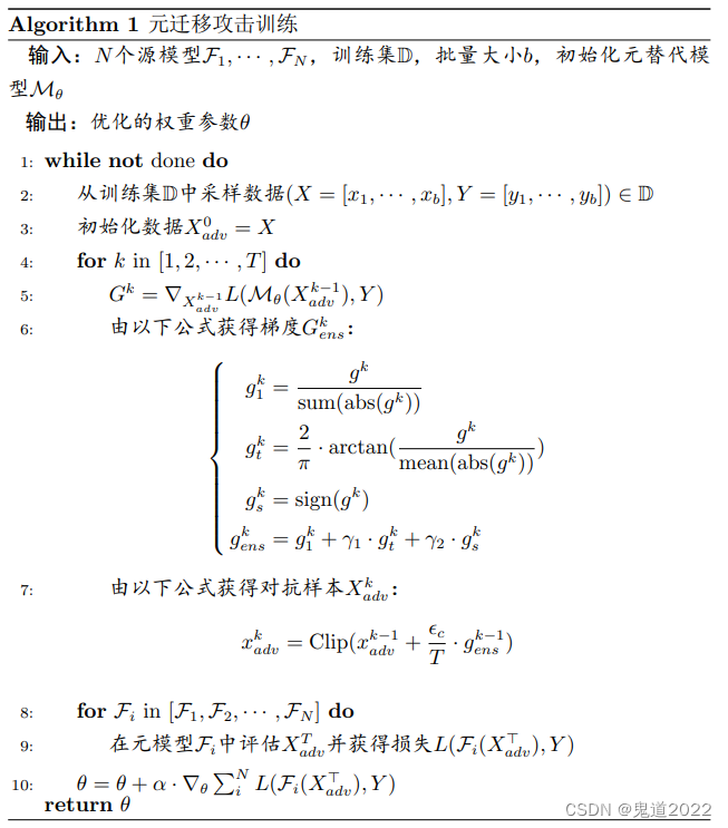

4 experimental result

  The table below shows that it is in Cifar-10 On dataset 8 Migration attack success rate of target networks , The meta agent model uses this 8 From the training of source model . The quantitative results in the following table show that , The method proposed in the paper MTA-PGD The performance of is much better than that of all previous methods , The migration success rate against attacks is significantly improved .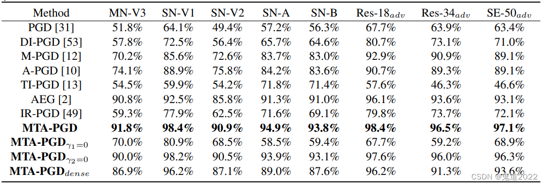

  The following figure shows the exploration in Cifar-10 On dataset , The relationship between the number of iterations in the anti attack algorithm and the success rate of migration attack . As you can see from the left half of the picture , Overall, the best number of iteration attacks is $T_t=7$; It can be seen from the right half of the picture , With the number of iterations $T_v$ An increase in , The success rate of migration attacks has also increased significantly .

  As shown in the figure below , Qualitative visualization results generated for different attack methods . You can intuitively find , The anti disturbance generated by the method proposed in this paper is more targeted , And the visually generated countermeasure sample is more similar to the original clean sample .

5 Code implementation

  Specific in the paper pytorch The simple code implementation of is as follows , The key steps involved in the algorithm flow chart of this paper are implemented , Parts of the dataset and model can be replaced by themselves .

iport torch
import torch.nn as nn
import torch.utils.data as Data
import numpy as np
import os
import torch.nn.functional as F
from copy import deepcopy

def generate_dataset(sample_num, class_num, X_shape):
        Label_list = []
        Sample_list = []
        for i in range(sample_num):
                y = np.random.randint(0, class_num)
                Label_list.append(y)
                Sample_list.append(np.random.normal(y, 0.2, X_shape))
        return torch.tensor(Sample_list).to(torch.float32), torch.tensor(Label_list).to(torch.int64)


class Normal_Dataset(Data.Dataset):
        def __init__(self, Numpy_Dataset):
                super(Normal_Dataset, self).__init__()
                self.data_tensor = Numpy_Dataset[0]
                self.target_tensor = Numpy_Dataset[1]

        def __getitem__(self, index):
                return self.data_tensor[index], self.target_tensor[index]

        def __len__(self):
                return self.data_tensor.size(0)

class Classifer(nn.Module):
        def __init__(self):
                super(Classifer, self).__init__()
                self.conv1 = nn.Conv2d(in_channels = 3, out_channels = 10, kernel_size = 9)  # 10, 36x36
                self.conv2 = nn.Conv2d(in_channels = 10, out_channels = 20, kernel_size = 17 ) # 20, 20x20
                self.fc1 = nn.Linear(20*20*20, 512)
                self.fc2 = nn.Linear(512, 7)

        def forward(self, x):
                in_size = x.size(0)
                out = self.conv1(x)
                out = F.relu(self.conv2(out))
                out = out.view(in_size, -1)
                out = F.relu(self.fc1(out))
                out = self.fc2(out)
                out = F.softmax(out, dim=1)
                return out

class MTA_training(object):
        def __init__(self, sml, dataloader, bs, msm, epsilon, iteration, gamma_1, gamma_2):
                self.source_model_list = source_model_list
                self.dataloader = dataloader
                self.batch_size = batch_size
                self.meta_surrogate_model = meta_surrogate_model
                self.epsilon = epsilon
                self.iteration = iteration
                self.dataloader = dataloader
                self.gamma1 = gamma1
                self.gamma2 = gamma2

        def single_attack(self, x, y, meta_surrogate_model):
                delta = torch.zeros_like(x)
                delta.requires_grad = True
                outputs = meta_surrogate_model(x + delta)
                loss = nn.CrossEntropyLoss()(outputs, y)
                loss.backward()
                grad = delta.grad.detach()
                ## The equation (4) of the paper
                g_1 = grad/torch.sum(torch.abs(grad))
                g_t = 2/np.pi * torch.atan(grad/torch.mean(torch.abs(grad)))
                g_s = torch.sign(grad)
                g_ens = g_1 + self.gamma1 * g_t + self.gamma2 * g_s
                ## The equation (5) of the paper
                x_adv = torch.clamp(x + self.epsilon/ self.iteration *  g_ens, 0 ,1)
                return x_adv

        def training(self, epoch):
                loss_fn = nn.CrossEntropyLoss()
                optim = torch.optim.SGD(meta_surrogate_model.parameters(), lr=0.001)
                for X, Y in self.dataloader:
                        theta_old_list = []
                        for parameter in  meta_surrogate_model.parameters():
                                theta_old_list.append(deepcopy(parameter.data))
                        X_adv = X
                        for k in range(self.iteration):
                                X_adv = self.single_attack(X_adv, Y, self.meta_surrogate_model)
                        loss = 0
                        for source_model in self.source_model_list:
                                outputs = source_model(X_adv)
                                loss += loss_fn(outputs , Y)
                        optim.zero_grad()
                        loss.backward()
                        optim.step()
                        for parameter_old, parameter in zip(theta_old_list, meta_surrogate_model.parameters()):
                                parameter.data = 2 * parameter.data - parameter_old.data

if __name__ == '__main__':
        batch_size = 2
        epsilon = 0.03
        iteration = 10
        epoch = 1
        gamma1 = 0.01
        gamma2 = 0.01
        numpy_dataset = generate_dataset(10, 7, (3, 44, 44))
        dataset = Normal_Dataset(numpy_dataset)
        dataloader = Data.DataLoader(
                                dataset = dataset,
                                batch_size = batch_size,
                                num_workers = 0,)

        source_model_list  = []
        source_model1 = Classifer()
        source_model2 = Classifer()
        source_model_list.append(source_model1)
        source_model_list.append(source_model2)
        meta_surrogate_model = Classifer()
        meta_training = MTA_training(source_model_list, dataloader, batch_size, meta_surrogate_model, epsilon, iteration, gamma1, gamma2)
        meta_training.training(10)