当前位置:网站首页>圖像識別與檢測--筆記
圖像識別與檢測--筆記
2022-07-03 07:26:00 【鹿銜草啊】
圖像識別與檢測
1.Variable
在 Torch 中的 Variable 就是一個存放會變化的值的地方(籃子)。 裏面的值會不停的變化。 裏面的值,就是Tensor張量(雞蛋)。
import torch
from torch.autograd import Variable # torch 中 Variable 模塊
# 准備雞蛋
tensor = torch.FloatTensor([[1,2],[3,4]])
# 把雞蛋放到籃子裏, requires_grad是參不參與誤差反向傳播, 要不要計算梯度
variable = Variable(tensor, requires_grad=True)

print("Tensor:\n" + str(tensor))
print("\n")
print("Variable:\n" + str(variable))

2. Variable 計算, 梯度
t_out = torch.mean(tensor*tensor)       # x^2
v_out = torch.mean(variable*variable)   # x^2
print(t_out)
print(v_out)
到目前為止, 我們看不出什麼不同, 但是時刻記住, Variable 計算時, 它在背景幕布後面一步步默默地搭建著一個龐大的系統, 叫做計算圖, computational graph. 這個圖是用來幹嘛的? 原來是將所有的計算步驟 (節點) 都連接起來, 最後進行誤差反向傳遞的時候, 一次性將所有 variable 裏面的修改幅度 (梯度) 都計算出來, 而 tensor 就沒有這個能力啦.
v_out = torch.mean(variable*variable)# 就是在計算圖中添加的一個計算步驟, 計算誤差反向傳遞的時候有他一份功勞, 我們就來舉個例子:
v_out.backward()    # 模擬 v_out 的誤差反向傳遞

# v_out = torch.mean(variable*variable) 這是定義
# v_out = 1/4 * sum(variable*variable) 這是計算圖中的 v_out的實際數學公式
# 針對於 v_out 的梯度就是:
# d(v_out)/d(variable) = 1/4*2*variable = variable/2
print("variable.grad:\n")
print(variable.grad)    # 初始 Variable 的梯度
3. 獲取 Variable 裏面的數據
直接print(variable)只會輸出 Variable 形式的數據, 在很多時候是用不了的(比如想要用 plt 畫圖), 所以我們要轉換一下, 將它變成 tensor 形式
print(variable)     # Variable 形式
print(variable.data)    # tensor 形式
print(variable.data.numpy())    # numpy 形式
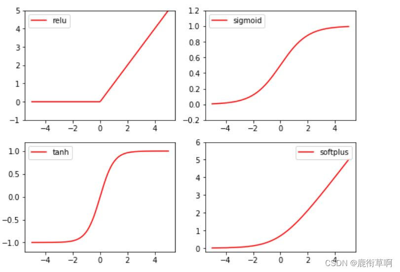
4. 激勵函數 (Activation)
常見的激勵函數:Relu, Sigmoid, Tanh, Softplus
import torch
import torch.nn.functional as F     # 激勵函數都在這
from torch.autograd import Variable

x = torch.linspace(-5, 5, 200)  # x data (tensor), shape=(100, 1)
x = Variable(x)
print(x.shape)

import matplotlib.pyplot as plt

plt.figure(1, figsize=(8, 6))
plt.subplot(221)
plt.plot(x_np, y_relu, c='red', label='relu')
plt.ylim((-1, 5))
plt.legend(loc='best')

plt.subplot(222)
plt.plot(x_np, y_sigmoid, c='red', label='sigmoid')
plt.ylim((-0.2, 1.2))
plt.legend(loc='best')

plt.subplot(223)
plt.plot(x_np, y_tanh, c='red', label='tanh')
plt.ylim((-1.2, 1.2))
plt.legend(loc='best')

plt.subplot(224)
plt.plot(x_np, y_softplus, c='red', label='softplus')
plt.ylim((-0.2, 6))
plt.legend(loc='best')

plt.show()
5. Regression
import torch
import torch.nn.functional as F     # 激勵函數都在這
import matplotlib.pyplot as plt
x = torch.unsqueeze(torch.linspace(-1, 1, 100), dim=1)  # x data (tensor), shape=(100, 1)
y = x.pow(2) + 0.2*torch.rand(x.size())                 # noisy y data (tensor), shape=(100, 1)

# 畫圖
plt.scatter(x.data.numpy(), y.data.numpy())
plt.show()

torch.unsqueeze(input, dim, out=None) 作用:擴展維度 返回一個新的張量,對輸入的既定比特置插入維度 1 注意: 返回張量與輸入張量共享內存,所以改變其中一個的內容會改變另一個
torch.linspace(start, end, steps=100, out=None) 返回一個1維張量,包含在區間start和end上均勻間隔的step個點。輸出張量的長度由steps决定。
參數: start (float) - 區間的起始點 end (float) - 區間的終點 steps (int) - 在start和end間生成的樣本數 out (Tensor, optional) - 結果張量
torch.rand(*sizes, out=None) → Tensor 返回一個張量,包含了從區間[0,1)的均勻分布中抽取的一組隨機數,形狀由可變參數sizes 定義。
參數: sizes (int…) – 整數序列,定義了輸出形狀 out (Tensor, optinal) - 結果張量
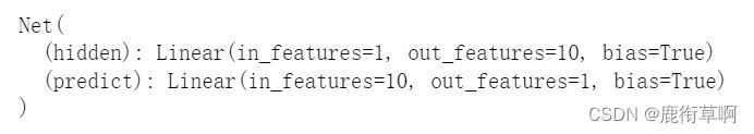
6. 建立神經網絡
class Net(torch.nn.Module):  # 繼承 torch 的 Module
    def __init__(self, n_feature, n_hidden, n_output):
        super(Net, self).__init__()     # 繼承 __init__ 功能
        # 定義每層用什麼樣的形式
        self.hidden = torch.nn.Linear(n_feature, n_hidden)   # 隱藏層線性輸出
        self.predict = torch.nn.Linear(n_hidden, n_output)   # 輸出層線性輸出

    def forward(self, x):   # 這同時也是 Module 中的 forward 功能
        # 正向傳播輸入值, 神經網絡分析出輸出值
        x = F.relu(self.hidden(x))      # 激勵函數(隱藏層的線性值)
        x = self.predict(x)             # 輸出值
        return x

net = Net(n_feature=1, n_hidden=10, n_output=1)

print(net)
net2 = torch.nn.Sequential(
    torch.nn.Linear(1, 10),
    torch.nn.ReLU(),
    torch.nn.Linear(10, 1)
)
print(net2)

7. 訓練網絡
# optimizer 是訓練的工具
optimizer = torch.optim.SGD(net.parameters(), lr=0.2)  # 傳入 net 的所有參數, 學習率
loss_func = torch.nn.MSELoss()      # 預測值和真實值的誤差計算公式 (均方差)

epochs = 200

plt.ion()   # 畫圖
plt.show()

for t in range(epochs):
    prediction = net(x)     # 喂給 net 訓練數據 x, 輸出預測值

    loss = loss_func(prediction, y)     # 計算兩者的誤差

    optimizer.zero_grad()   # 清空上一步的殘餘更新參數值
    loss.backward()         # 誤差反向傳播, 計算參數更新值
    optimizer.step()        # 將參數更新值施加到 net 的 parameters 上

    #畫圖
    if t % 5 == 0:
        # plot and show learning process
        plt.cla()
        plt.scatter(x.data.numpy(), y.data.numpy())
        plt.plot(x.data.numpy(), prediction.data.numpy(), 'r-', lw=5)
        plt.text(0.5, 0, 'Loss=%.4f' % loss.data.numpy(), fontdict={
    'size': 20, 'color':  'red'})
        plt.pause(0.1)
边栏推荐
- 论文学习——鄱阳湖星子站水位时间序列相似度研究
- 最全SQL与NoSQL优缺点对比
- Split small interface
- TCP cumulative acknowledgement and window value update
- Operation and maintenance technical support personnel have hardware maintenance experience in Hong Kong
- Introduction of buffer flow
- PgSQL converts string to double type (to_number())
- Le Seigneur des anneaux: l'anneau du pouvoir
- TypeScript let与var的区别
- [solved] unknown error 1146
猜你喜欢
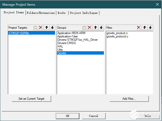
【开发笔记】基于机智云4G转接板GC211的设备上云APP控制

New stills of Lord of the rings: the ring of strength: the caster of the ring of strength appears

Basic components and intermediate components

VMware network mode - bridge, host only, NAT network
专题 | 同步 异步
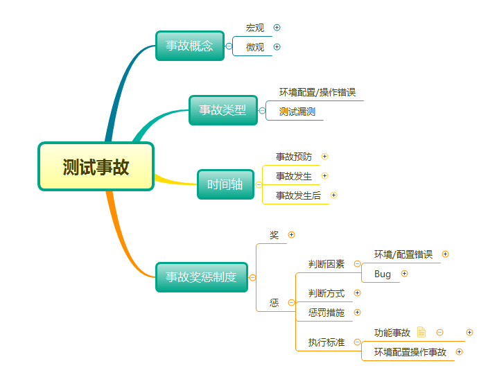
Take you through the whole process and comprehensively understand the software accidents that belong to testing
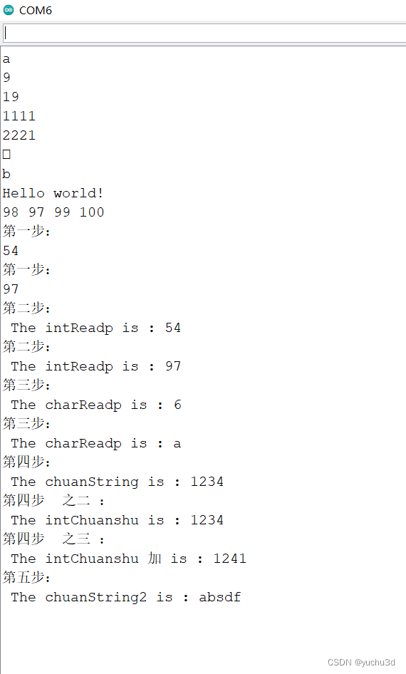
Summary of Arduino serial functions related to print read
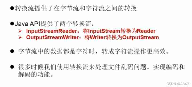
Introduction of transformation flow
VMWare网络模式-桥接,Host-Only,NAT网络
![[set theory] Stirling subset number (Stirling subset number concept | ball model | Stirling subset number recurrence formula | binary relationship refinement relationship of division)](/img/d8/b4f39d9637c9886a8c81ca125d6944.jpg)
[set theory] Stirling subset number (Stirling subset number concept | ball model | Stirling subset number recurrence formula | binary relationship refinement relationship of division)
随机推荐
Responsive MySQL of vertx
Leetcode 198: 打家劫舍
4EVERLAND:IPFS 上的 Web3 开发者中心,部署了超过 30,000 个 Dapp!
Store WordPress media content on 4everland to complete decentralized storage
Web router of vertx
IP home online query platform
Warehouse database fields_ Summary of SQL problems in kingbase8 migration of Jincang database
[HCAI] learning summary OSI model
TCP cumulative acknowledgement and window value update
Hash table, generic
Advanced API (byte stream & buffer stream)
Use of other streams
Distributed lock
Advanced API (batch image Download & socket dialog)
"Baidu Cup" CTF game 2017 February, Web: blast-1
LeetCode
SecureCRT password to cancel session recording
The difference between typescript let and VaR
Book recommendation~
【开发笔记】基于机智云4G转接板GC211的设备上云APP控制