Li Hongyi machine learning team learning punch in activity day04 - Introduction to deep learning and back propagation mechanism

Write it at the front

I signed up for a team learning activity , Today's task is deep learning , There is little contact before deep learning , You can study hard this time .

Reference video :https://www.bilibili.com/video/av59538266
Reference notes ：https://github.com/datawhalechina/leeml-notes

Deep learning Introduction

The three steps of deep learning

deep learning There are generally three parts ：

• step1: neural network (Neural network)
• step2: Model to evaluate (Goodness of function)
• step3: Choose the best function (Pick best function)
  

step1: neural network

Neuron ： Nodes in Neural Networks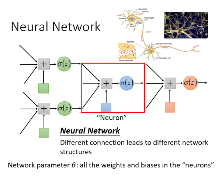

Neural networks have many different connections , This will produce different structures .

Complete feedforward neural network
Concept ： feedforward (feedforward) It can also be called forward , From the signal flow direction to understand is the input signal into the network , Signal flow is Individual Of , That is, the signal flows from the previous layer to the next layer , All the way to the output layer , There is no connection between any two layers feedback (feedback), That is, the signal does not return from the next layer to the previous layer .

For example, the input (1,-1) and (-1,0) Result ：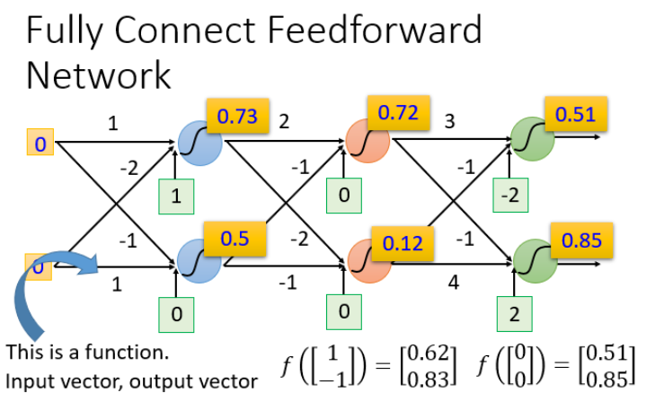

We can set the parameters of the above structure to different numbers , Just different functions （function）. These possible functions （function） Together, it is a set of functions （function set）.

Full link and feedforward understanding

• Input layer （Input Layer）：1 layer
• Hidden layer （Hidden Layer）：N layer
• Output layer （Output Layer）：1 layer
  

Fully connected understanding : because layer And layer2 There are connections between Liangliang , So it's called full link (Fully Connect)
Feedforward understanding : Because the direction of transmission is from back to front , So it's called Feedforward.

Deep understanding
What does that mean Deep Well ？Deep = Many hidden layer. How many floors can there be ？
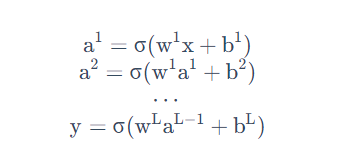
As the number of layers increases , Lower error rate , And then the amount of computation increases , It's usually more than a billion calculations . use Matrix operations It can speed up the calculation .

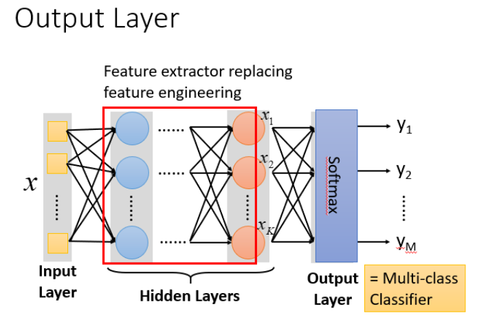
The essence ： Feature transformation through hidden layer
The hidden layer is replaced by the original feature engineering by feature extraction , So in the last hidden layer, the output is a new set of features （ Equivalent to black box operation ） And for the output layer , In fact, the output of the previous hidden layer is regarded as the input （ The best set of features obtained by feature extraction ） And then through a multi classifier （ It can be softmax function ） Get the final output y.

step2: Model to evaluate

Examples of losses ：

For losses , We don't just need to calculate the amount of data , It's about calculating the loss of all the training data as a whole , And then add up the loss of all the training data , Get an overall loss L.
Evaluation of the model . We usually use the loss function to reflect the quality of the model , For neural networks , It is generally used ** Cross entropy (cross entropy)** Function to calculate .

step3: Choose the best function

gradient descent

Specific process ：$\theta$ It's a set of parameters with weights and deviations , Find an initial value at random , Next, calculate the partial differential corresponding to each parameter , Get a set of partial differential $\nabla L$ It's gradient , With these partial differentials , You can update the gradient constantly to get new parameters , It's going on over and over again , You can get the best parameters to minimize the loss function .

Back propagation

The best way to calculate the loss in neural network clock is back propagation , You can use TensorFlow, theano, Pytorch Etc. frame calculation .

1. Loss function (Loss function) It's defined on a single training sample , That is to calculate the error of a sample ,
2. Cost function (Cost function) It's defined throughout the training set , That is, the average of the sum of the errors of all samples .
3. The total loss function (Total loss function) It's defined on the whole training set , That is, the total error of all samples , That is to evaluate the value that we need to minimize back propagation .
   

For a neuron (Neuron) Analyze

Forward part

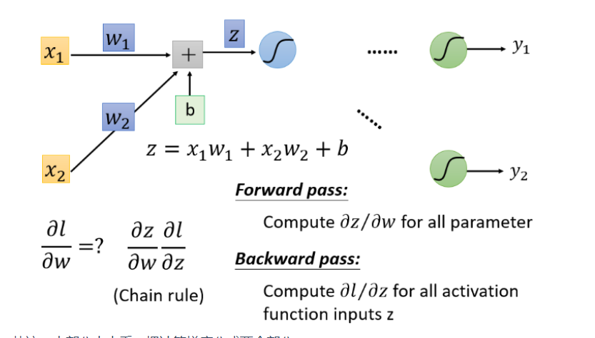
According to the differential principle ,$\frac{\partial z}{\partial w_1}=x_1$, $\frac{\partial z}{\partial w_2}=x_2$

Reverse part

final result ：

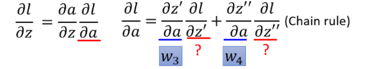
understand ： But you can imagine looking at this thing from another angle , Now there's another neuron , hold forward The process is reversed ,
among ${\sigma }^{\prime }(z)$ Is constant , Because it has been determined when it propagates forward .

if $\frac{\partial l}{\partial z^{\prime }}$ and $\frac{\partial l}{\partial z^{\prime \prime }}$ It's the last hidden layer , Then direct calculation can get the result

if $\frac{\partial l}{\partial z^{\prime }}$ and $\frac{\partial l}{\partial z^{\prime \prime }}$ The last hidden layer , You need to calculate it all the way back through the chain rule

summary

Our goal is to calculate $\frac{\partial z}{\partial w}$(Forward pass part ) And calculation KaTeX parse error: Undefined control sequence: \patial at position 19: …ac{\partial l}{\̲p̲a̲t̲i̲a̲l̲ ̲z}(Backward pass Part of ), And then $\frac{\partial z}{\partial w}$ and KaTeX parse error: Undefined control sequence: \patial at position 19: …ac{\partial l}{\̲p̲a̲t̲i̲a̲l̲ ̲z} Multiply and you get
$\frac{\partial l}{\partial w}$, You can get all the parameters in the neural network , Then use gradient descent to continuously update , Get the loss minimum function .