Thesis reading (53):universal advantageous perturbations

1 summary

  

1.1 subject

  2017CVPR： Universal anti disturbance (Universal adversarial perturbations)

1.2 Method

   The point is as follows ：
  1） It shows that for a given cutting-edge neural network classifier , Only a universal and minimal disturbance can cause high probability misclassification of natural images ;
  2） Put forward a kind of A systematic algorithm for computing general perturbations , It is shown that the most advanced deep neural network is very susceptible to this disturbance , And the human eye can almost detect ;
  3） Further empirical analysis of these universal perturbations , And show their application in neural network Good generalization performance ;
  4） The existence of universal perturbation reveals the important geometric correlation between the high-dimensional decision boundaries of classifiers . It further outlines the potential security vulnerabilities in a single direction in the input space , Attackers may use these directions to destroy classifiers on most natural images .

1.3 Code

  Tensorflow：https://github.com/LTS4/universal
  Torch：https://github.com/NetoPedro/Universal-Adversarial-Perturbations-Pytorch

1.4 Bib

@inproceedings{
    Moosavi:2017:17651773,
author		=	{
    Seyed-Mohsen Moosavi-Dezfooli and Alhussein Fawzi and Omar Fawzi and Pascal Frossard},
title		=	{
    Universal adversarial perturbations},
booktitle	=	{
    {
    IEEE} Conference on Computer Vision and Pattern Recognition},
pages		=	{
    1765--1773},
year		=	{
    2017}
}

2 Universal disturbance

   Make $\mu$ Indicates that the image is in space ${\mathbb{R}}^d$ The distribution on ,$\hat{k}$ Is a tool for acquiring images $x\in {\mathbb{R}}^d$ Assessment tags $\hat{k}(x)$ Classifier . The purpose of this paper is Find a perturbation vector $v\in {\mathbb{R}}^b$, It can fool $\hat{k}$ In most cases $\mu$ On the data points of ：
$$\hat{k}(x+v)\ne \hat{k}(x)fo{r}^{\prime \prime }mos{t}^{\prime \prime }x\sim \mu .$$ The universal disturbance represents a fixed disturbance independent of the image , It will cause the labels of most images sampled from the data distribution to change . Here we focus on distribution $\mu$ Represents a natural image set , So it contains a lot of variability . In this case , Universal small perturbations that mislead most images will be discovered . seek $v$ Need to meet the following constraint ：
  1）$\Vert v{\Vert }_p\le \xi$ ;
  2）${\mathbb{P}}_{x\sim \mu }(\hat{k}(x+v)\ne \hat{k}(x))\ge 1-\delta$.
here $\xi$ Used to control the $v$ The intensity of ,$\delta$ Used to control the misleading rate .

Algorithm

   Make $X=\{x_1,\dots ,x_m\}$ It means that it obeys the distribution $\mu$ A collection of images . Based on constraints and optimization objectives , The algorithm will be in $X$ Iterate over and build the universal perturbation step by step , Such as chart 2. In each iteration , Calculate the current perturbation point $x_i+v$ The minimum disturbance sent to the decision boundary of the classifier $v_i$, And it is aggregated to the current instance of universal disturbance .

chart 2： The semantic representation of the proposed algorithm in computing universal perturbations . spot $x_1$、$x_2$, as well as $x_3$ In superposition state , Different classification areas $\mathcal{A}$ Displayed in different colors . The purpose of the algorithm is to find the minimum disturbance , Make a point of $x_i+v$ Move out of the correct classification area

   Assume that the current generic perturbation $v$ Data points cannot be fooled $x_i$, We solve the following optimization problems to find data points that can be cheated $x_i$ Additional perturbation of the minimum norm of $v_i$：
$$\Delta v_i\leftarrow \underset{r}{\mathrm{argmin}}\Vert r{\Vert }_{2}s.t.\hat{k}(x_i+v+r)\ne {\hat{x}}_i.\text{\hspace{1em}(1)}$$ To ensure that constraints are met $\Vert v{\Vert }_p\le \xi$, The updated universal perturbation is further projected to a radius of $\xi$、 Center in $0$ Of ${\ell }_p$ On the ball . therefore , Projection operations are defined as ：
$${\mathcal{P}}_{p,\xi }(v)=\underset{v^{\prime }}{\mathrm{argmin}}\Vert v-v^{\prime }{\Vert }_{2}s.t.\Vert v^{\prime }{\Vert }_p\le \xi .$$ then , The update rule changes to $v\leftarrow {\mathcal{P}}_{p,\xi }(v+\Delta v_i)$. The data set $X$ The quality of the universal disturbance will be improved by the multiple transmission of . The algorithm will be applied to perturbed data sets $X_v:=\{x_1+v,\dots ,x_m+v\}$ The fooling rate of exceeds the threshold $1-\delta$ Stop when ：
$$\text{Err}(X_v):=\frac{1}{m}\sum _{i=1}^m{1}_{\hat{k}(x_i+v)\ne \hat{k}(x_i)}\ge 1-\delta .$$ Algorithm 1 Show more details .$X$ Number of data points in $m$ It doesn't take much to compute a pair of global distributions $\mu$ Effective universal perturbation . Special ,$m$ It can be set to a value much smaller than the training sample .

   The proposed algorithm involves solving the formula at each transfer 1 At most of the optimization problems in $m$ An example , Here the Deepfool To deal with this problem efficiently . It is worth noting that , Algorithm 1 It is not possible to find a minimum universal perturbation that fools as many sample points as possible , Only one perturbation with a sufficiently small norm can be found .$X$ Different random shuffles will naturally lead to various universal perturbations that satisfy the required constraints $v$.

3 Universal disturbance and depth network

   This section analyzes how the leading edge deep learning classifier responds to Algorithm 1 Robustness of universal perturbations in .
   First experiment in , Evaluate different algorithms in ILSVRC 2012 Verify the universal perturbation on the data set , And show Fooling rate , That is, the proportion of the image label that will change after the universal disturbance . The experiment will take place in $X=10000$;$p=2$ and $p=\infty$ Proceed under , The corresponding $\xi$ Respectively $2000$ and $10$. These values are chosen to obtain perturbations whose norm is significantly smaller than the image norm , So when added to a natural image , Disturbances are imperceptible . surface 1 It shows the experimental results . Each result is reported in the set used to calculate the disturbance $X$ And validation set （ It is not used in the calculation of general disturbance ）. The results show that the universal perturbation has a high fooling rate .

   chart 3 It shows GoogleNet Visualization results of disturbed images . in the majority of cases , Universal disturbances are imperceptible , Such image perturbations effectively fool many leading edge classifiers .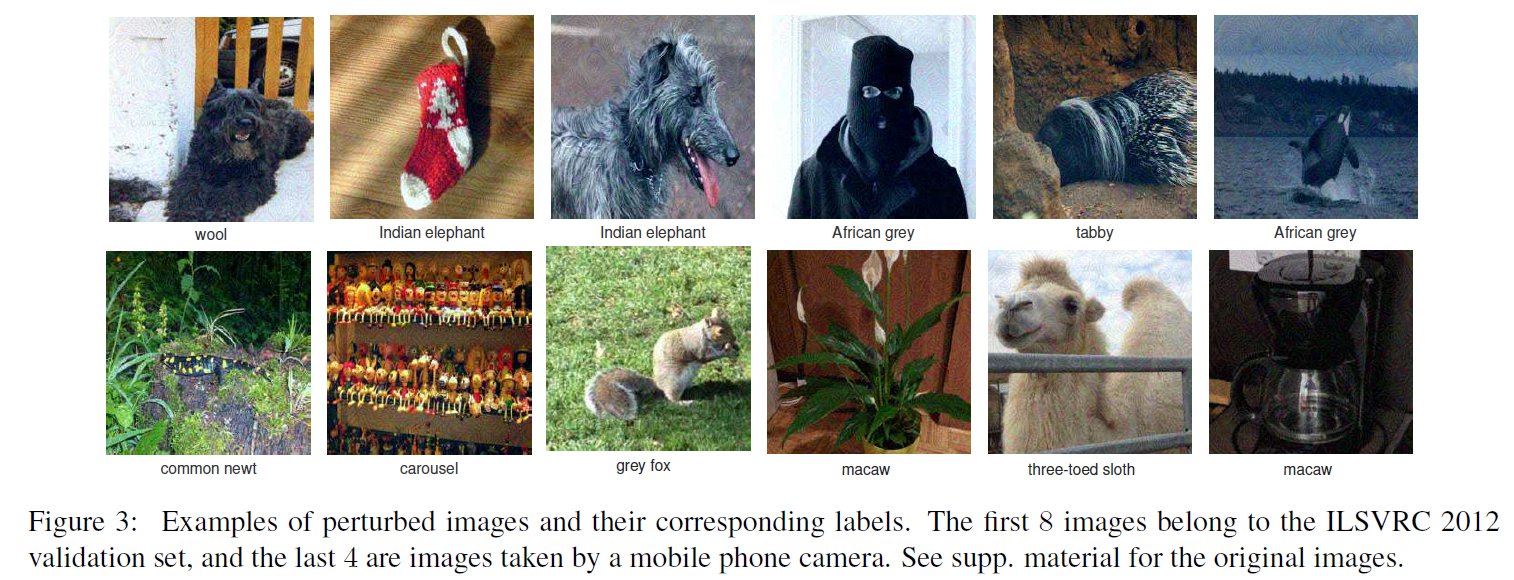

   chart 4 The universal perturbation results of different networks are shown . It should be noted that , Universal perturbations are not unique , Because many different universal perturbations can be generated for the same network ( Both satisfy the two required constraints ).

   chart 5 It shows $X$ Different universal perturbations under different random shuffles . The results show that the universal perturbations are different in similar modes . Besides , This is also confirmed by calculating the normalized inner product between two pairs of disturbed images , Because the normalized inner product does not exceed 0.1, This shows that different universal perturbations can be found .

   The second experiment Used to verify $X$ The influence of the size of the on the universal disturbance . chart 6 It shows GoogleNet In different $X$ The fooling rate . Experiments show that only in $X=500$ when , The fooling rate can reach 30%.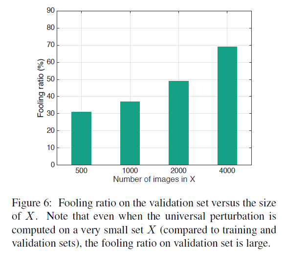

3.1 Cross model universality

   After calculating the disturbance at an unknown data point , It can be proved that they are universal across models , That is, on a special network such as VGG-19 The disturbance of training , It can still be on another network, such as GoogleNet Effective on . surface 2 Shows the cross model fooling rate .

3.2 Visualization of universal disturbance performance

   In order to visually demonstrate the utility of universal perturbations on natural images , We will ImageNet The label distribution on the validation set is visualized ： Undirected graph $G=(V,E)$, Where the fixed point represents the label , edge $e=(i\to j)$ Indicates that the icon label changes from... After the disturbance is applied $i$ Be misled into $j$, Such as chart 7.

3.3 Fine tuning of universal perturbations

   It is used to test the performance of the network after fine-tuning using the disturbed image . Use VGG-F framework , And fine tune the network based on the modified training set , The universal perturbation is added to a small number of clean training samples ： For each training point , With 0.5 The probability of adding generic perturbations , And the original sample is 0.5 Probability retention . To explain the diversity of universal perturbations ,10 Two precomputed universal perturbations will be randomly selected . The network will be fine tuned five times on the modified dataset . Set during fine adjustment $p=\infty$ And $\xi =10$. The results showed that the fooling rate decreased .

4 The vulnerability of neural networks

   This section is used to illustrate the vulnerability of neural networks to pervasive disturbances . First, compare it with other types of disturbances , Explain the uniqueness of universal perturbations , Include ：
  1） Random disturbance ;
  2） Against disturbance ;
  3）$X$ Up against the sum of disturbances ;
  4） The mean value of the image .
   chart 8 Different disturbances are shown $\xi$ And ${\ell }_2$ The fooling rate under the norm . Specially , The great difference between the universal disturbance and the random disturbance indicates that , Universal perturbations utilize some geometric correlations between different parts of the classifier decision boundary . in fact , If the direction of the decision boundary near different data points is completely irrelevant ( And it has nothing to do with the distance of decision boundary ), Then the norm of the optimal universal perturbation will be equal to that of the random perturbation . further , The random perturbation norm required to deceive a particular data point is precisely expressed as $\Theta (\sqrt{d}\Vert r{\Vert }_2)$, among $d$ Is the dimension of the input space . about ImageNet Classification task , Yes $\sqrt{d}\Vert r{\Vert }_2\approx 2\times 10^4$. For most data points , This is better than the universal perturbation ($\xi =2000$) One order of magnitude larger . therefore , The substantial difference between random disturbance and universal disturbance indicates that the geometry of decision boundary explored at present is redundant .

   For each image in the validation set $x$, The anti disturbance vector obtained is $r(x)=\underset{r}{\mathrm{argmin}}\Vert r{\Vert }_{2}s.t.\hat{k}(x+r)\ne \hat{k}(x)$. Obviously $r(x)$ The decision boundary with the classifier is $x+r(x)$ Orthogonal at . therefore $r(x)$ To capture decision boundaries in $x$ Local geometric features in adjacent regions . In order to quantify the correlation between different regions of the classifier decision boundary , Defines the validation set $n$ Normal vector matrix of decision boundary near data points ：
$$N=\left[\frac{r(x_1)}{\Vert r(x_1){\Vert }_2}\cdots \frac{r(x_n)}{\Vert r(x_n){\Vert }_2}\right]$$ For binary classifier , The decision boundary is a hyperplane 、$N$ The rank of is 1, And all normal vectors are collinear . In order to more generally capture the correlation in the decision boundary of complex classifiers , We calculate the matrix $N$ The singular value of . adopt CaffeNet Calculated matrix $N$ The singular value of is as follows chart 9. The figure shows when $N$ Column the singular values obtained when sampling randomly and uniformly from the unit sphere . Although the singular value of the latter decays slowly , but $N$ The singular value of decays rapidly , This proves that the decision boundary of the deep network has large correlation and redundancy . More precisely , This indicates that there is a low dimension $d^{\prime }\ll d$ Subspace $S$, It contains most of the normal vectors of the decision boundary in the region around the natural image . Suppose that the existence of universal perturbations that fool most natural images is due to the existence of such a low dimensional subspace , The subspace captures the correlation between different regions of the decision boundary . in fact , This subspace “ collect ” The normals of decision boundaries in different regions are given , Therefore, the disturbance belonging to this subspace may deceive the data points . To test this hypothesis , We choose a norm $\xi =2000$ The random vector of , Of the former 100 A subspace traversed by a singular vector $S$, And calculate the fooling rate of different image sets ( That is, a group that has not been used to calculate SVD Image ). This disturbance can deceive the near 38% Image , So it shows that in this subspace $S$ The random direction in is obviously better than the random disturbance ( This disturbance can only deceive 10% The data of ).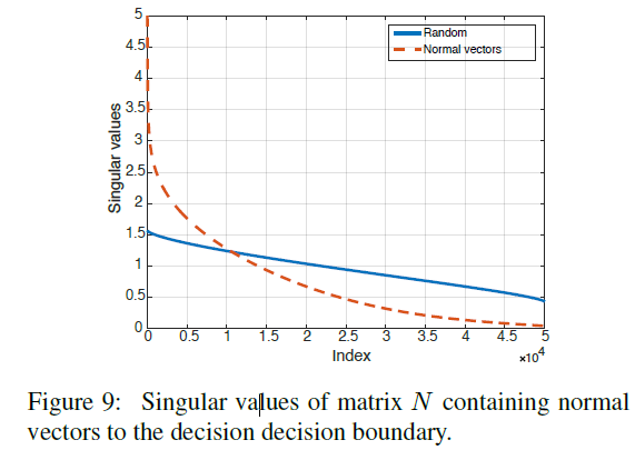

   chart 10 It shows the relevance subspace in the capture decision boundary $S$. It should be noted that , The existence of this low dimensional subspace explains chart 6 The surprising generalization properties of the universal perturbations obtained in , Among them, people can use very few images to construct relatively generalized universal perturbations .
   Different from the above experiment , The proposed algorithm does not select a random vector in this subspace , Instead, choose a specific direction to maximize the overall fooling rate . This explains the use of $S$ Random vector strategy and algorithm in 1 The difference between the obtained fooling rates .