当前位置：网站首页>特征工程特征降维

特征工程特征降维

2022-06-11 04:11:00 【落花雨时】

一、降维

1.1 定义

降维是指在某些限定条件下，降低随机变量(特征)个数，得到一组“不相关”主变量的过程

降低随机变量的个数
相关特征(correlated feature)
- 相对湿度与降雨量之间的相关
- 等等

正是因为在进行训练的时候，我们都是使用特征进行学习。如果特征本身存在问题或者特征之间相关性较强，对于算法学习预测会影响较大

1.2 降维的两种方式

特征选择
主成分分析（可以理解一种特征提取的方式）

二、特征选择

2.1 定义

数据中包含冗余或无关变量（或称特征、属性、指标等），旨在从原有特征中找出主要特征。

在这里插入图片描述

2.2 方法

Filter(过滤式)：主要探究特征本身特点、特征与特征和目标值之间关联
- 方差选择法：低方差特征过滤
- 相关系数
Embedded (嵌入式)：算法自动选择特征（特征与目标值之间的关联）
- 决策树:信息熵、信息增益
- 正则化：L1、L2
- 深度学习：卷积等

2.3 低方差特征过滤

删除低方差的一些特征，前面讲过方差的意义。再结合方差的大小来考虑这个方式的角度。

特征方差小：某个特征大多样本的值比较相近
特征方差大：某个特征很多样本的值都有差别

2.3.1 API

sklearn.feature_selection.VarianceThreshold(threshold = 0.0)
- 删除所有低方差特征
- Variance.fit_transform(X)
  - X:numpy array格式的数据[n_samples,n_features]
  - 返回值：训练集差异低于threshold的特征将被删除。默认值是保留所有非零方差特征，即删除所有样本中具有相同值的特征。

2.3.2 数据计算

我们对某些股票的指标特征之间进行一个筛选，除去’index,‘date’,'return’列不考虑（这些类型不匹配，也不是所需要指标）

一共这些特征

pe_ratio,pb_ratio,market_cap,return_on_asset_net_profit,du_return_on_equity,ev,earnings_per_share,revenue,total_expense

index,pe_ratio,pb_ratio,market_cap,return_on_asset_net_profit,du_return_on_equity,ev,earnings_per_share,revenue,total_expense,date,return
0,000001.XSHE,5.9572,1.1818,85252550922.0,0.8008,14.9403,1211444855670.0,2.01,20701401000.0,10882540000.0,2012-01-31,0.027657228229937388
1,000002.XSHE,7.0289,1.588,84113358168.0,1.6463,7.8656,300252061695.0,0.326,29308369223.2,23783476901.2,2012-01-31,0.08235182370820669
2,000008.XSHE,-262.7461,7.0003,517045520.0,-0.5678,-0.5943,770517752.56,-0.006,11679829.03,12030080.04,2012-01-31,0.09978900335112327
3,000060.XSHE,16.476,3.7146,19680455995.0,5.6036,14.617,28009159184.6,0.35,9189386877.65,7935542726.05,2012-01-31,0.12159482758620697
4,000069.XSHE,12.5878,2.5616,41727214853.0,2.8729,10.9097,81247380359.0,0.271,8951453490.28,7091397989.13,2012-01-31,-0.0026808154146886697

分析：

1、初始化VarianceThreshold,指定阀值方差

2、调用fit_transform

def variance_demo():
    """ 删除低方差特征——特征选择 :return: None """
    data = pd.read_csv("factor_returns.csv")
    print(data)
    # 1、实例化一个转换器类
    transfer = VarianceThreshold(threshold=1)
    # 2、调用fit_transform
    data = transfer.fit_transform(data.iloc[:, 1:10])
    print("删除低方差特征的结果：\n", data)
    print("形状：\n", data.shape)

    return None

返回结果：

            index  pe_ratio  pb_ratio    market_cap  \
0     000001.XSHE    5.9572    1.1818  8.525255e+10   
1     000002.XSHE    7.0289    1.5880  8.411336e+10    
...           ...       ...       ...           ...   
2316  601958.XSHG   52.5408    2.4646  3.287910e+10   
2317  601989.XSHG   14.2203    1.4103  5.911086e+10   

      return_on_asset_net_profit  du_return_on_equity            ev  \
0                         0.8008              14.9403  1.211445e+12   
1                         1.6463               7.8656  3.002521e+11    
...                          ...                  ...           ...   
2316                      2.7444               2.9202  3.883803e+10   
2317                      2.0383               8.6179  2.020661e+11   

      earnings_per_share       revenue  total_expense        date    return  
0                 2.0100  2.070140e+10   1.088254e+10  2012-01-31  0.027657  
1                 0.3260  2.930837e+10   2.378348e+10  2012-01-31  0.082352  
2                -0.0060  1.167983e+07   1.203008e+07  2012-01-31  0.099789   
...                  ...           ...            ...         ...       ...  
2315              0.2200  1.789082e+10   1.749295e+10  2012-11-30  0.137134  
2316              0.1210  6.465392e+09   6.009007e+09  2012-11-30  0.149167  
2317              0.2470  4.509872e+10   4.132842e+10  2012-11-30  0.183629  

[2318 rows x 12 columns]

删除低方差特征的结果：
 [[  5.95720000e+00   1.18180000e+00   8.52525509e+10 ...,   1.21144486e+12
    2.07014010e+10   1.08825400e+10]
 [  7.02890000e+00   1.58800000e+00   8.41133582e+10 ...,   3.00252062e+11
    2.93083692e+10   2.37834769e+10]
 [ -2.62746100e+02   7.00030000e+00   5.17045520e+08 ...,   7.70517753e+08
    1.16798290e+07   1.20300800e+07]
 ..., 
 [  3.95523000e+01   4.00520000e+00   1.70243430e+10 ...,   2.42081699e+10
    1.78908166e+10   1.74929478e+10]
 [  5.25408000e+01   2.46460000e+00   3.28790988e+10 ...,   3.88380258e+10
    6.46539204e+09   6.00900728e+09]
 [  1.42203000e+01   1.41030000e+00   5.91108572e+10 ...,   2.02066110e+11
    4.50987171e+10   4.13284212e+10]]
形状：
 (2318, 8)

2.4 相关系数

主要实现方式：
- 皮尔逊相关系数
- 斯皮尔曼相关系数

2.4.1 皮尔逊相关系数(Pearson Correlation Coefficient)

1. 作用

反映变量之间相关关系密切程度的统计指标

2. 公式计算案例(了解，不用记忆)

公式

在这里插入图片描述

举例

比如说我们计算年广告费投入与月均销售额

在这里插入图片描述

那么之间的相关系数怎么计算

在这里插入图片描述

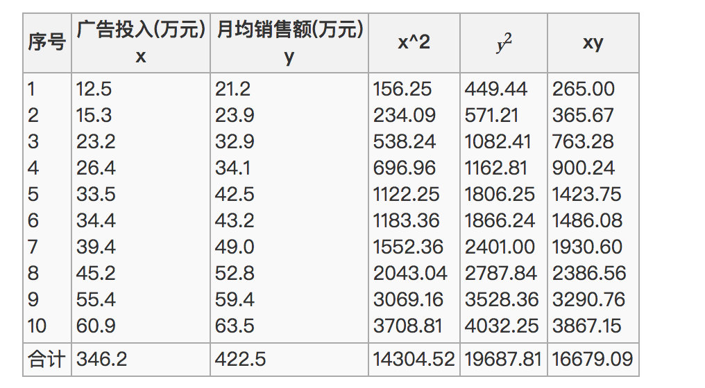
最终计算：
在这里插入图片描述

= 0.9942

所以我们最终得出结论是广告投入费与月平均销售额之间有高度的正相关关系。

3. 特点

相关系数的值介于–1与+1之间，即–1≤ r ≤+1。其性质如下：

当r>0时，表示两变量正相关，r<0时，两变量为负相关
当|r|=1时，表示两变量为完全相关，当r=0时，表示两变量间无相关关系
当0<|r|<1时，表示两变量存在一定程度的相关。且|r|越接近1，两变量间线性关系越密切；|r|越接近于0，表示两变量的线性相关越弱
一般可按三级划分：|r|<0.4为低度相关；0.4≤|r|<0.7为显著性相关；0.7≤|r|<1为高度线性相关

4. api

from scipy.stats import pearsonr
- x : (N,) array_like
- y : (N,) array_like Returns: (Pearson’s correlation coefficient, p-value)

5. 案例

from scipy.stats import pearsonr

x1 = [12.5, 15.3, 23.2, 26.4, 33.5, 34.4, 39.4, 45.2, 55.4, 60.9]
x2 = [21.2, 23.9, 32.9, 34.1, 42.5, 43.2, 49.0, 52.8, 59.4, 63.5]

pearsonr(x1, x2)

结果

(0.9941983762371883, 4.9220899554573455e-09)

2.4.2 斯皮尔曼相关系数(Rank IC)

1.作用：

反映变量之间相关关系密切程度的统计指标

2.公式计算案例(了解，不用记忆)

公式:

在这里插入图片描述

n为等级个数，d为二列成对变量的等级差数

举例:

在这里插入图片描述

3.特点

斯皮尔曼相关系数表明 X (自变量) 和 Y (因变量)的相关方向。如果当X增加时， Y 趋向于增加, 斯皮尔曼相关系数则为正
与之前的皮尔逊相关系数大小性质一样，取值 [-1, 1]之间

斯皮尔曼相关系数比皮尔逊相关系数应用更加广泛

4.api

from scipy.stats import spearmanr

5.案例

from scipy.stats import spearmanr

x1 = [12.5, 15.3, 23.2, 26.4, 33.5, 34.4, 39.4, 45.2, 55.4, 60.9]
x2 = [21.2, 23.9, 32.9, 34.1, 42.5, 43.2, 49.0, 52.8, 59.4, 63.5]

spearmanr(x1, x2)

结果

SpearmanrResult(correlation=0.9999999999999999, pvalue=6.646897422032013e-64)

三、主成分分析

原理建议参考：https://blog.csdn.net/weixin_43312354/article/details/105653308

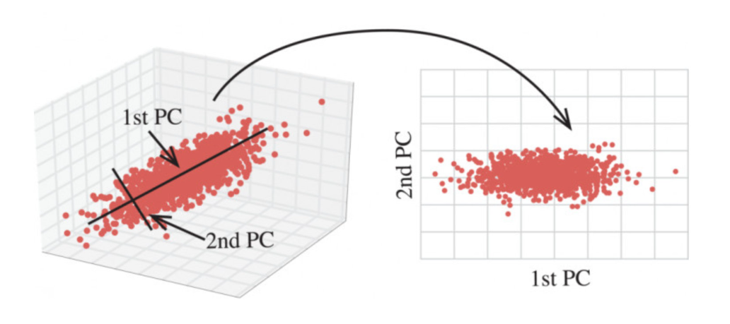
3.1 什么是主成分分析(PCA)

定义：高维数据转化为低维数据的过程，在此过程中可能会舍弃原有数据、创造新的变量
作用：是数据维数压缩，尽可能降低原数据的维数（复杂度），损失少量信息。
应用：回归分析或者聚类分析当中

对于信息一词，在决策树中会进行介绍

那么更好的理解这个过程呢？我们来看一张图

在这里插入图片描述

3.2 API

sklearn.decomposition.PCA(n_components=None)
- 将数据分解为较低维数空间
- n_components:
  - 小数：表示保留百分之多少的信息
  - 整数：减少到多少特征
- PCA.fit_transform(X) X:numpy array格式的数据[n_samples,n_features]
- 返回值：转换后指定维度的array

3.3 数据计算

先拿个简单的数据计算一下

from sklearn.decomposition import PCA

def pca_demo():
    """ 对数据进行PCA降维 :return: None """
    data = [[2,8,4,5], [6,3,0,8], [5,4,9,1]]

    # 1、实例化PCA, 小数——保留多少信息
    transfer = PCA(n_components=0.9)
    # 2、调用fit_transform
    data1 = transfer.fit_transform(data)

    print("保留90%的信息，降维结果为：\n", data1)

    # 1、实例化PCA, 整数——指定降维到的维数
    transfer2 = PCA(n_components=3)
    # 2、调用fit_transform
    data2 = transfer2.fit_transform(data)
    print("降维到3维的结果：\n", data2)

    return None

返回结果：

保留90%的信息，降维结果为：
 [[ -3.13587302e-16   3.82970843e+00]
 [ -5.74456265e+00  -1.91485422e+00]
 [  5.74456265e+00  -1.91485422e+00]]
降维到3维的结果：
 [[ -3.13587302e-16   3.82970843e+00   4.59544715e-16]
 [ -5.74456265e+00  -1.91485422e+00   4.59544715e-16]
 [  5.74456265e+00  -1.91485422e+00   4.59544715e-16]]

原网站

版权声明
本文为[落花雨时]所创，转载请带上原文链接，感谢
https://blog.csdn.net/mengxianglong123/article/details/125214755

当前位置：网站首页>特征工程特征降维

特征工程特征降维

文章目录

一、降维

1.1 定义

1.2 降维的两种方式

二、特征选择

2.1 定义

2.2 方法

2.3 低方差特征过滤

2.3.1 API

2.3.2 数据计算

2.4 相关系数

2.4.1 皮尔逊相关系数(Pearson Correlation Coefficient)

1. 作用

2. 公式计算案例(了解，不用记忆)

3. 特点

4. api

5. 案例

2.4.2 斯皮尔曼相关系数(Rank IC)

1.作用：

2.公式计算案例(了解，不用记忆)

3.特点

4.api

5.案例

三、主成分分析

3.1 什么是主成分分析(PCA)

3.2 API

3.3 数据计算

边栏推荐

猜你喜欢

随机推荐

当前位置：网站首页>特征工程 特征降维

特征工程 特征降维

文章目录

一、降维

1.1 定义

1.2 降维的两种方式

二、特征选择

2.1 定义

2.2 方法

2.3 低方差特征过滤

2.3.1 API

2.3.2 数据计算

2.4 相关系数

2.4.1 皮尔逊相关系数(Pearson Correlation Coefficient)

1. 作用

2. 公式计算案例(了解，不用记忆)

3. 特点

4. api

5. 案例

2.4.2 斯皮尔曼相关系数(Rank IC)

1.作用：

2.公式计算案例(了解，不用记忆)

3.特点

4.api

5.案例

三、 主成分分析

3.1 什么是主成分分析(PCA)

3.2 API

3.3 数据计算

边栏推荐

猜你喜欢

随机推荐

当前位置：网站首页>特征工程特征降维

特征工程特征降维

三、主成分分析