当前位置:网站首页>Machine Learning - Notes and Implementation of Linear Regression, Logistic Regression Problems
Machine Learning - Notes and Implementation of Linear Regression, Logistic Regression Problems
2022-07-31 07:45:00 【Miracle Fan】
回归问题
概述:
A regression problem is all about predicting the value of a continuous problem,比如……,
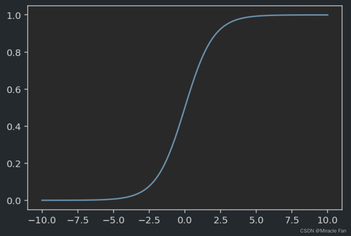
And if the above regression problem,利用Sigmoid函数(Logistic 回归),The ability to turn a predicted value into a probability of judging whether or not something can be done,Change the continuous value obtained by regression to (0,1)之间的概率,It can then be used to deal with binary classification problems
一元线性回归
线性回归方程为:
y ^ = a x + b \hat{y} =ax+b y^=ax+b
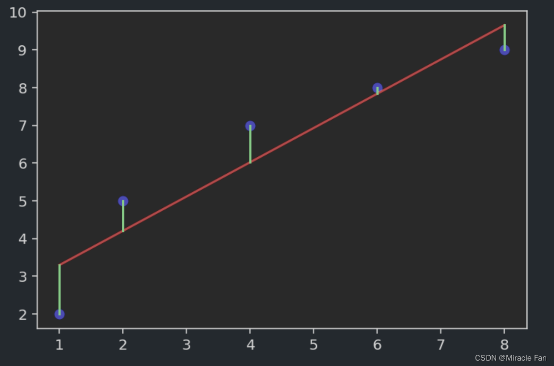
For example, given a set of data,The following scatterplot can be obtained.
x=np.array([1,2,4,6,8])
y=np.array([2,5,7,8,9])

for linear regression,Equivalent to we fit a straight line,It is a good way to connect the various samples in the above figure,But in general, the perfect fitting effect cannot be achieved,Just wish it was as shown in the image below,The green line represents the error between the predicted point and the true point,We want the error to be as small as possible,That is, a better fitting effect can be achieved.
y_pred=lambda x: a*x+b
plt.scatter(x,y,color='b')
plt.plot(x,y_pred(x),color='r')
plt.plot([x,x], [y,y_pred(x)], color='g')
plt.show()
That is, a loss function can be defined:
L = 1 n ∑ i = 1 n ( y i − y p r e d i ) L=\frac{1}{n}\sum^n_{i=1}(y^i-y_{pred}^i) L=n1i=1∑n(yi−ypredi)
But if you choose this function,When we do the error calculation,In some cases the predicted value is larger than the true value,In some cases the predicted value is smaller than the true value.则会导致 y − y p r e d y-y_{pred} y−ypred出现正、negative case,when adding them together,will cause mutual cancellation,So here we need to use the mean squared loss function:
L = 1 n ∑ i = 1 n ( y i − y p r e d i ) 2 L=\frac{1}{n}\sum^n_{i=1}(y^i-y_{pred}^i)^2 L=n1i=1∑n(yi−ypredi)2
Substitute into the fitting equation:
L = 1 n ∑ i = 1 n ( y i − a x i − b ) 2 L=\frac{1}{n}\sum^n_{i=1}(y^i-ax^i-b)^2 L=n1i=1∑n(yi−axi−b)2
Use the least squares method to derive the rule:
a = ∑ i = 1 n ( x i − x ˉ ) ( y i − y ˉ ) ∑ i = 1 n ( x i − x ˉ ) 2 b = y ˉ − a x ˉ a=\frac{\sum_{i=1}^n(x_i-\bar{x})(y^i-\bar{y})}{\sum_{i=1}^n(x^i-\bar{x})^2}\\ b=\bar{y}-a\bar{x} a=∑i=1n(xi−xˉ)2∑i=1n(xi−xˉ)(yi−yˉ)b=yˉ−axˉ
def Linear_Regression(x,y):
    x_mean=np.mean(x)
    y_mean=np.mean(y)
    # num=np.sum((x-np.tile(x_mean,x.shape))*(y-np.tile(y_mean,y.shape)))
    num=np.sum((x-x_mean)*(y-y_mean))
    den=np.sum((x-x_mean)**2)
    a=num/den
    b=y_mean-a*x_mean
    return a,b
由于numpy的广播机制,Not necessary herex_mean的维度进行调整.
多元线性回归
对于多元线性回归,其一般表达式为:
y = θ 0 + θ 1 x 1 + θ 2 x 2 + ⋯ + θ n x n y=\theta_0+\theta_1x_1+\theta_2x_2+\dots+\theta_nx_n y=θ0+θ1x1+θ2x2+⋯+θnxn
This formula can be simplified to :
Y = θ ⋅ X Y=\theta \cdot X Y=θ⋅X
X = ( 1 x 11 ⋯ x 1 p 1 x 21 ⋯ x 2 p ⋮ ⋮ ⋱ ⋮ 1 x n 1 ⋯ x n p ) X=\left(\begin{array}{cccc} 1 & x_{11} & \cdots & x_{1 p} \\ 1 & x_{21} & \cdots & x_{2 p} \\ \vdots & \vdots & \ddots & \vdots \\ 1 & x_{n 1} & \cdots & x_{n p} \end{array}\right) X=⎝⎛11⋮1x11x21⋮xn1⋯⋯⋱⋯x1px2p⋮xnp⎠⎞
θ = ( θ 0 θ 1 θ 2 … θ n ) \theta=\begin{pmatrix} \theta_0\\ \theta_1\\ \theta_2\\ \dots \\ \theta _n \end{pmatrix} θ=⎝⎛θ0θ1θ2…θn⎠⎞
而对于 θ \theta θ的求解,Use the least squares method used above,可以得到:
θ = ( X i T X i ) − 1 X i T y \theta=(X_i^TX_i)^{-1}X_i^Ty θ=(XiTXi)−1XiTy
#Generates a column for manipulating intercept values
ones = np.ones((X_train.shape[0], 1))
#在horizentalstack in the direction
X_b = np.hstack((ones, X_train)) # 将XThe matrix is converted to the first column1,其余不变的X_b矩阵
theta = linalg.inv(X_b.T.dot(X_b)).dot(X_b.T).dot(y_train)
interception = theta[0]
coef =theta[1:]
logistic回归
简单的logisticsRegression is the addition of linear regressionSigmoid函数,Implement compression of prediction results,keep it there(0,1)It can also be understood as a probability value,Then usually with 0.5作为分界线,概率大于0.5则为类别1反之为0.
It is used to utilize probability problems obtained by linear regressionsigmoidThe output of the function is a class question.
p = 1 1 + e − z p=\frac{1}{1+e^{-z}} p=1+e−z1
- z:Usually a linear regression equation
- p:The predicted probability,Determine which category belongs to by dividing line
梯度下降
Gradient descent is mainly used to optimize the loss function,找到lossThe parameter value with the smallest value.
For example, suppose a loss function is
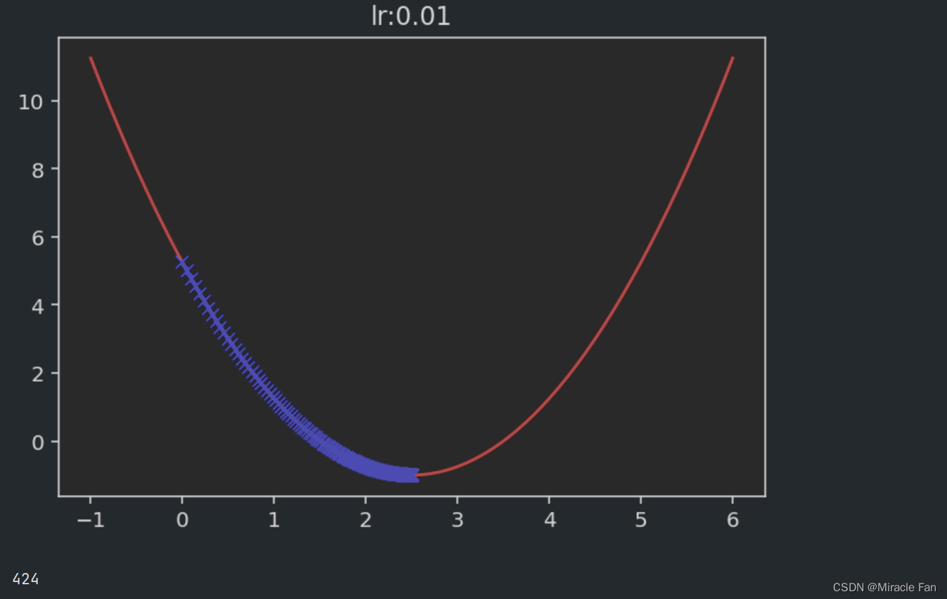
L = ( x − 2.5 ) 2 − 1 L=(x-2.5)^2-1 L=(x−2.5)2−1
Then define its loss function and its derivative.
def J(theta):
    try:
        return (theta-2.5)**2-1
    except:
        return float('inf')
def dJ(theta):
    return 2*(theta-2.5)
每一次迭代
θ = θ + η d J θ \theta=\theta+\eta\frac{dJ}{\theta} θ=θ+ηθdJ
def CalGradient(eta):
    theta = 0.0
    theta_history = [theta]
    epsilon = 1e-8#Used to finally terminate the computation of gradient descent
    while True:
        gradient = dJ(theta)
        last_theta = theta
        theta = theta - eta * gradient
        theta_history.append(theta)
        if (abs(J(theta) - J(last_theta)) < epsilon):
            break

    plt.title('lr:' + str(eta))
    plt.plot(x, J(x), color='r')
    plt.plot(np.array(theta_history), J(np.array(theta_history)), color='b', marker='x')
    plt.show()
    print(len(theta_history))
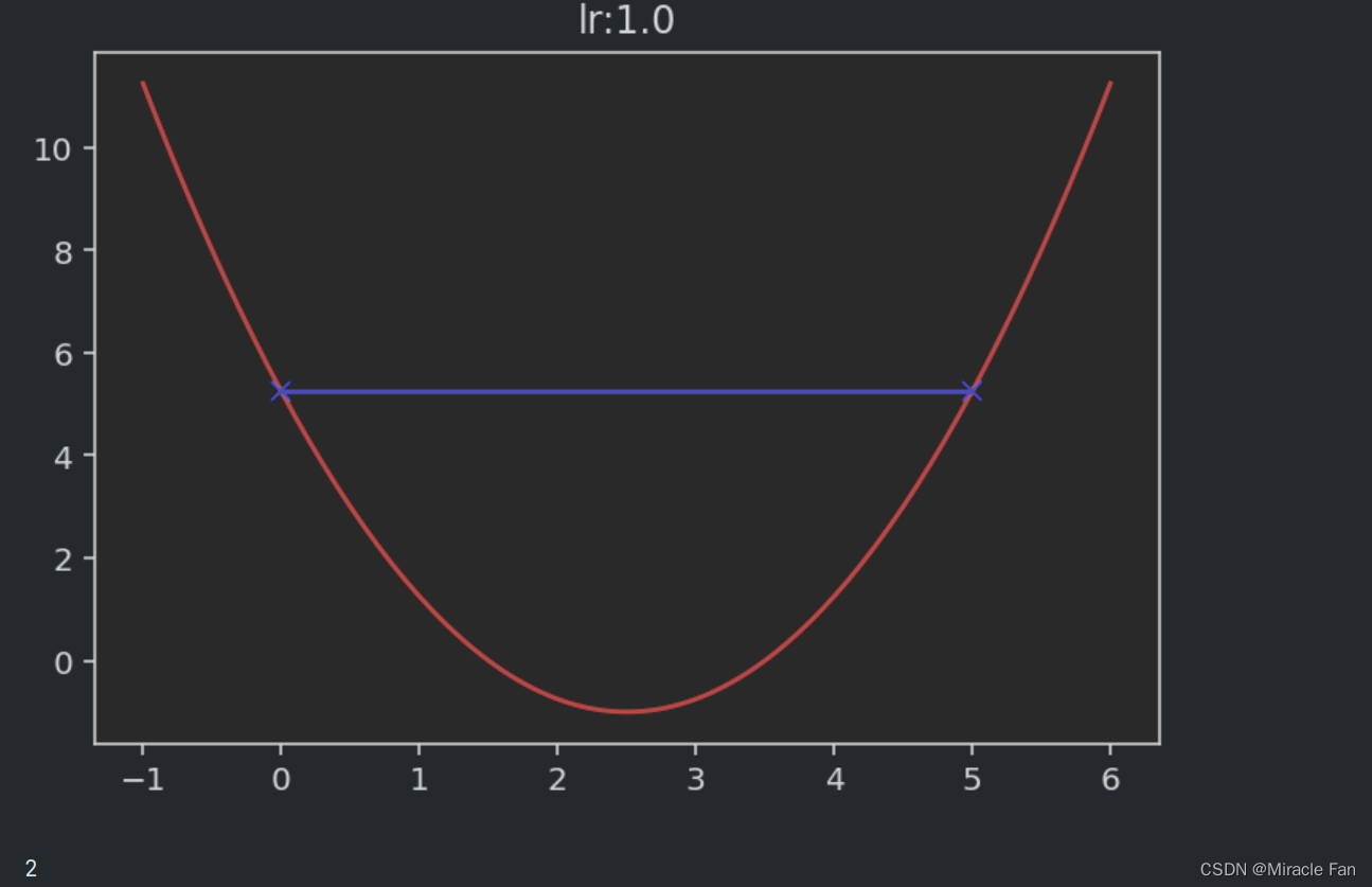
It is relevant when taking different learning rates,The drop chart is shown below.The learning rate is generally in 0~1之间,As shown in the figure below when the learning rate is1时,Convergence has not been reached,And when the learning rate is greater than 1时,It will show a divergent state.

Logistic回归的损失函数
LogisticRegression The expression after incorporating linear regression is shown below:
p = 1 1 + e − θ X p=\frac{1}{1+e^{-\theta X}} p=1+e−θX1
对于Logistic回归,The logarithmic loss function is generally used,Compute the parameters.
c o s t = { − log ( p p r e d ) i f y = 1 − log ( 1 − p p r e d ) i f y = 0 cost=\left \{\begin{matrix} -\log^{(p_{pred})} \quad if &y=1\\ -\log^{(1-p_{pred})} \quad if &y=0 \end{matrix}\right. cost={ −log(ppred)if−log(1−ppred)ify=1y=0
With a little tidying up, a loss function can be synthesized:
c o s t = − y log ( p p r e d ) − ( 1 − y ) log ( 1 − p p r e d ) cost=-y\log(p_{pred})-(1-y)\log({1-p_{pred}}) cost=−ylog(ppred)−(1−y)log(1−ppred)
import numpy as np

class LogisticRegression:

    def __init__(self):
        self.coef_ = None
        self.intercept_ = None
        self._theta = None

    def _sigmoid(self, x):
        y = 1.0 / (1.0 + np.exp(-x))
        return y

    def fit(self, x_train, y_train, eta=0.01, n_iters=1e4):
        assert x_train.shape[0] == y_train.shape[0], 'The number of training set and its label length samples needs to be consistent'

        def J(theta, x, y):
            p_pred = self._sigmoid(x.dot(theta))
            try:
                return -np.sum(y * np.log(p_pred) + (1 - y) * np.log(1 - p_pred)) / len(y)
            except:
                return float('inf')

        def dJ(theta, x, y):
            x = self._sigmoid(x.dot(theta))
            return x.dot(x - y) / len(x)

            # Simulate gradient descent

        def gradient_descent(X_b, y, initial_theta, eta, n_iters=1e4, epsilon=1e-8):
            theta = initial_theta
            i_iter = 0
            while i_iter < n_iters:
                gradient = dJ(theta, X_b, y)
                last_theta = theta
                theta = theta - eta * gradient
                i_iter += 1
                if (abs(J(theta, X_b, y) - J(last_theta, X_b, y)) < epsilon):
                    break
            return theta

        X_b = np.hstack([np.ones((len(x_train), 1)), x_train])
        initial_theta = np.zeros(X_b.shape[1])  # 列向量
        self._theta = gradient_descent(X_b, y_train, initial_theta, eta, n_iters)
        self.intercept_ = self._theta[0]  # 截距
        self.coef_ = self._theta[1:]  # 维度
        return self

    def predict_proba(self, X_predict):
        X_b = np.hstack([np.ones((len(X_predict), 1)), X_predict])
        return self._sigmoid(X_b.dot(self._theta))

    def predict(self, X_predict):
        proba = self.predict_proba(X_predict)
        return np.array(proba > 0.5, dtype='int')
边栏推荐
猜你喜欢


随机推荐
SQL Server Datetime2数据类型
2022.07.26_每日一题
tidyverse笔记——dplyr包
多进程全局变量失效、变量共享问题
Yu Mr Series 】 【 2022 July 022 - Go Go teaching course of container in the dictionary
Gradle remove dependency demo
【C语言项目合集】这十个入门必备练手项目,让C语言对你来说不再难学!
DAY18:XSS 漏洞
Leetcode952. Calculate maximum component size by common factor
2022.07.20_Daily Question
van-uploader上传图片,使用base64回显无法预览的问题
2022.07.15_每日一题
2022.07.13 _ a day
2022.7.29 Array
【Star项目】小帽飞机大战(七)
DAY18: Xss Range Clearance Manual
'vite' is not an internal or external command, nor is it a runnable program or batch file.
Tasks and task switching
超级详细的mysql数据库安装指南
opencv、pil和from torchvision.transforms的Resize, Compose, ToTensor, Normalize等差别