10. DCN introduction

Preface

Conventional CTR Predictive models require a lot of Feature Engineering , time-consuming ; introduce DNN after , Rely on the strong learning ability of neural network , It can realize automatic learning feature combination to a certain extent . however DNN The disadvantage of is the unexplainability caused by the combination of implicit learning features , And inefficient learning ( Not all feature combinations are useful ).
In the beginning FM The inner product of hidden vectors is used to model combined features ;FFM On this basis, we introduce field The concept of , For different field Use different hidden vectors on . however , Both of them are aimed at modeling low-order feature combination .
and DNN The learned features are highly nonlinear high-order composite features , The meaning is very difficult to explain .

1、 DCN Introduce

DCN Full name Deep & Cross Network, It's Google and Stanford University 2017 Proposed in for Ad Click Prediction Model of .DCN(Deep Cross Network) stay It is very efficient to learn the combined features of a specific order , And no feature engineering is required , The additional complexity introduced is also minimal .

2、DCN Model structure

DCN The architecture diagram is shown in the figure above ： The beginning is Embedding and stacking layer, Then parallel Cross Network and Deep Network, And finally Combination Layer hold Cross Network and Deep Network Results of Output.

2.1 Embedding and Stacking Layer

• Why Embed？

  • stay web-scale Recommendation systems such as CTR Under estimation , Most of the input features are category features , The usual solution is one-hot, however one-hot After that, the input feature dimension is very high and very sparse .
  • So there is Embedding To greatly reduce the input dimension , That's all binary features convert to dense vectors with real values.
  • Embedding The operation is actually using a matrix and one-hot The subsequent inputs are multiplied , It can also be regarded as a query （lookup）. This Embedding The matrix is the same as other parameters in the network , You need to learn along with the network .

• Why Stack？
  Finished processing categorical features , There are also continuous features that do not deal with that . So after we normalize continuous features , And embedded vectors stacking together , You get the original input ：

2.2 Cross Network

Cross Network It is the core of the whole thesis . It is designed to efficiently learn combinatorial features , The key is how to do it efficiently feature crossing. Formalize it as follows ：

xl and xl+1 They are the first l Tier and tier l+1 layer cross layer Output ,wl and bl Is the connection parameter between the two layers . Note that all variables in the above formula are column vectors ,W It's also a column vector , It's not a matrix .

• How to understand ？
  It's not hard ,xl+1 = f(xl, wl, bl) + xl. The output of each layer , Are the output of the previous layer plus feature crossing f. and f Is to fit the residual between the output of this layer and the output of the previous layer . in the light of one cross layer The visualization is as follows ：

• High-degree Interaction Across Features:

Cross Network The special network structure makes cross feature The order of increases with layer depth To increase by . Relative to input x0 Come on , One l Layer of cross network Of cross feature The order of is l+1.

• Complexity analysis ：
  Let's say there are Lc layer cross layer, Start input x0 The dimensions are d. So the whole cross network The number of parameters of is :

Because every floor W and b All are d Dimensional .
It can be found from the above formula that , Complexity is the input dimension d The linear function of . So compared to deep network,cross network The complexity introduced is negligible . That's the guarantee DCN The complexity and DNN It's a level of . The paper says ,Cross Network The reason why we can effectively learn combination features , Because of x0 * xT The rank of is 1, So that we can get all the... Without calculating and storing the whole matrix cross terms.
however , Precisely because cross network The relatively few parameters lead to its limited expression ability , In order to be able to learn highly nonlinear combinatorial features ,DCN Parallel introduces Deep Network.

2.3 Deep Network

This part is nothing special , It is a fully connected neural network with forward propagation , We can calculate the number of parameters to estimate the complexity . Assume that the input x0 Dimension for d, Altogether Lc Layer neural networks , The number of neurons in each layer is m individual . Then the total parameter or complexity is ：

2.4 Combination Layer

Combination Layer hold Cross Network and Deep Network The output is spliced , Then after a weighted sum, we get logits, And then pass by sigmoid Function to get the final prediction probability . Formalize it as follows ：

p Is the final prediction probability ;XL1 yes d Dimensional , Express Cross Network Final output of ;hL2 yes m Dimensional , Express Deep Network Final output of ;Wlogits yes Combination Layer The weight of ; Last pass sigmoid function , Get the final prediction probability .

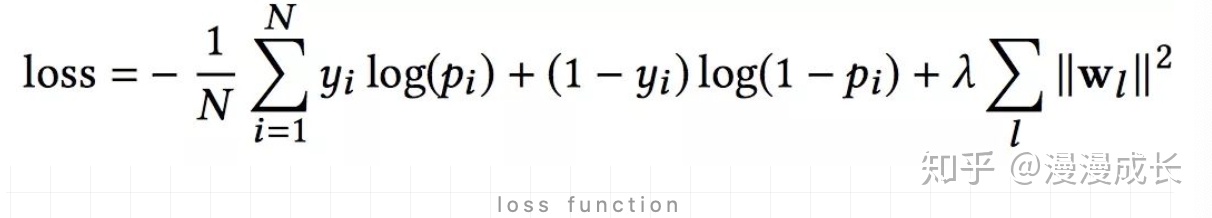
The loss function uses... With regular terms log loss, Formalize it as follows ：

in addition , in the light of Cross Network and Deep Network,DCN They train together , In this way, the network can know the existence of another network .

3、 example

The code used next is mainly open source DeepCTR, Corresponding API The documentation can be read here
https://deepctr-doc.readthedocs.io/en/latest/Examples.html

import pandas as pd
from sklearn.preprocessing import LabelEncoder, MinMaxScaler
from sklearn.model_selection import train_test_split
from deepctr.models.dcn import DCN
from deepctr.feature_column import SparseFeat, DenseFeat, get_feature_names

data = pd.read_csv('./criteo_sample.txt')

sparse_features = ['C' + str(i) for i in range(1, 27)]
dense_features = ['I' + str(i) for i in range(1, 14)]

data[sparse_features] = data[sparse_features].fillna('-1', )
data[dense_features] = data[dense_features].fillna(0, )
target = ['label']

for feat in sparse_features:
    lbe = LabelEncoder()
    data[feat] = lbe.fit_transform(data[feat])

mms = MinMaxScaler(feature_range=(0, 1))
data[dense_features] = mms.fit_transform(data[dense_features])

sparse_feature_columns = [SparseFeat(feat, vocabulary_size=data[feat].nunique(), embedding_dim=4)
                          for i, feat in enumerate(sparse_features)]
#  perhaps hash,vocabulary_size Usually bigger , To avoid hash Conflict too much 
# sparse_feature_columns = [SparseFeat(feat, vocabulary_size=1e6,embedding_dim=4,use_hash=True)
#                            for i,feat in enumerate(sparse_features)]#The dimension can be set according to data
dense_feature_columns = [DenseFeat(feat, 1)
                         for feat in dense_features]

dnn_feature_columns = sparse_feature_columns + dense_feature_columns
linear_feature_columns = sparse_feature_columns + dense_feature_columns
feature_names = get_feature_names(linear_feature_columns + dnn_feature_columns)

train, test = train_test_split(data, test_size=0.2)

train_model_input = {name: train[name].values for name in feature_names}
test_model_input = {name: test[name].values for name in feature_names}

model = DCN(linear_feature_columns, dnn_feature_columns, task='binary')
model.compile("adam", "binary_crossentropy",
              metrics=['binary_crossentropy'], )

history = model.fit(train_model_input, train[target].values,
                    batch_size=256, epochs=10, verbose=2, validation_split=0.2, )
pred_ans = model.predict(test_model_input, batch_size=256)

4、 summary

DCN The characteristics are as follows ：

• Use cross network, Apply... At every level feature crossing. Efficient learning bounded degree Combination features . There is no need for artificial feature Engineering .
• The network structure is simple and efficient . Polynomial complexity is determined by layer depth decision .
• Compared with DNN,DCN Of logloss A lower , And the number of parameters is nearly one order of magnitude less .