当前位置：网站首页>Matlab [functions and images]

name call	contain The righteous	name call	contain The righteous	name call	contain The righteous
abs	The absolute value	asin	Anti sine	coth	Hyperbolic cotangent
exp	Index	acos	Arccosine	asinh	Anti hyperbolic sine
log	logarithm	atan	Anyway	acosh	Anti hyperbolic cosine
log10	10 Base logarithm	acot	Inverse cotangent	atanh	Anti hyperbolic tangent
log2	2 Base logarithm	sec	Secant	acoth	Inverse hyperbolic cotangent
pow2	2 The next power	csc	Cosecant	sech	Hyperbolic secant
sqrt	square root	asec	Anyway	csch	Hyperbolic cosecant
sin	sine	acsc	Anti cosecant	asech	Inverse hyperbolic secant
cos	cosine	sinh	Hyperbolic sine	acsch	Inverse hyperbolic cosecant
tan	tangent	cosh	Hyperbolic cosine
cot	Cotangent	tanh	Hyperbolic tangent

A simple example

1. Several writing methods of function representation

1. Define function variables as symbolic variables

syms x
fx=sqrt(1+x^2);

2. Use function command

function f=myfun(x)
f=(3-2.*x).^2.*x;

3. Using anonymous functions

[email protected](x) (x+10)

Two 、 Representation of piecewise functions

Use if-else Judgment can help us implement piecewise functions

function y= w(x)
  if x<0
      y=x+2;
  else
      y=x-3;
  end
end

3、 ... and 、 Use functions to draw graphics

1. Draw the function image of absolute value

# Clear the screen 
clear
# Take us x Set as variable 
syms x 
# Use anonymous methods to create our y
[email protected](x) abs(x);
# Use fplot, The first parameter is our method , The second parameter is our argument x The scope of the 
fplot(y,[-5,5])
# Keep our current graph from being reset 
hold on
# Set up our x Axis labels 
xlabel('x')
# Set up our y Axis labels 
ylabel('y')
# Set the label of our whole picture 
title('y|x|')

2. Draw an image of the rounding function

clear
syms x 
[email protected](x) floor(x);
fplot(y,[-5,5])
hold on
xlabel('x')
ylabel('y')

3. Drawing piecewise functions

clear
syms x y
[email protected](x) 2*sqrt(x);
# The third parameter is our drawing line style 
fplot(y1,[0,1], '-b')
hold on
[email protected](x) 1+x;
fplot(y2,[1,5], '--og')
# Set our legend 
legend('y=2*sqrt(x) ', 'y=1+x');
title(' Piecewise functions ')
xlabel('x')
ylabel('y')
# Set the range of our axes , The first and second parameters represent x The scope of the shaft 
# The third and fourth parameters represent y The scope of the shaft 
axis([0,5,0,5])

4. Draw a normal distribution curve

clear
x=-2:0.01:2;
y=(1/sqrt(2*pi))*exp(-x.^2/2);
#plot The function takes our x,y Pass it in and you can draw 
plot(x,y)
title(' Normal distribution curve ')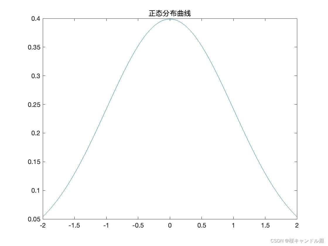

5. Draw symbolic functions

clear
# Set us x Maximum value of axis 
xm=5;
# Set up our x Take all from the minimum value to the maximum value , And the interval is 0.01
x=-xm:0.01:xm;
#sign For our symbolic function 
y=sign(x);
# Will we x==0 Time null , Breakpoints will be formed 
y(x==0)=nan;
figure
# drawing , And set the width of our line to 2
plot(x,y,'LineWidth',2)
hold on
# Draw us 0,1 Place and 0,-1 Two hollow points at 
plot(0,1,'o',0,-1,'o');
# Point a point at our origin 
plot(0,0,'.','MarkerSize',24)
# Name the title 
title(' Symbolic function ','FontSize',16)
# Set up our x Shaft labels and y Axis labels 
xlabel('\itx','FontSize',16)
ylabel('\ity','FontSize',16)
# Draw gridlines 
grid on
axis([-xm,xm,-2,2])

6. Draw the cube root of positive and negative numbers

clear
% Set up x Of max Range                                   
xm=5;
% Set up our x The range of is from -xm To xm, Spacing is 0.01                                  
x=-xm:0.01:xm;   
% Let's multiply each element of the vector y=x The third root of                       
y=x.^(1/3);  
% mapping                           
figure  
% Create icons with two rows and one column , And put the picture we want to draw next in the first chart                                
subplot(2,1,1)   
% Use plot Method , And our corresponding x,y Value in , And set the width of our drawn line to 2                      
plot(x,y,'LineWidth',2)     
% Draw our grid lines            
grid on   
% Title our chart                              
title(' Incorrect open cube for negative numbers ','FontSize',16)
% Separate our x,y The axis is titled 
xlabel('\itx','FontSize',16)           
ylabel('\ity','FontSize',16)    
% Because we are drawing 1 It is found that the negative range of our cube root is incorrect ,
% So we need to take out our symbols separately , Then multiply by the absolute value of our original function        
y=sign(x).*abs(x).^(1/3);              
subplot(2,1,2)                                
plot(x,y,'LineWidth',2)               
grid on                              
title(' Negative numbers open the cube correctly ','FontSize',16) 
xlabel('\itx','FontSize',16)          
ylabel('\ity','FontSize',16)

7. How to draw a graph with infinity

If we draw our tan(x) This happens to function

clear;
x=-5:0.01:5;
y=tan(x);
plot(x,y,'LineWidth',2)

Use ezplot, Pass our formula into , And then into our scope , You can draw pictures .

clear;
syms x
y=tan(x);
y=inline(y);
ezplot(y,[-2*pi,2*pi]);

8. How to draw implicit functions

ezplot You can also draw implicit function images

clear;
syms x
ezplot("x^2/4+y^2/6=1");

Use axis([x Shaft Downline ,x Axis upper limit ,y Axis lower limit ,y Axis upper limit ]) You can specify the range of our coordinate axes
axis("equal") So that our axis x,y Isometric axis

How to set up ezplot The format of

Take us ezplot Then the result is passed to a parameter , And then use our set To set our ezplot The type of drawing

clear;
syms x
h=ezplot("x^2/4+y^2/6=1");
set(h,'color','r','LineWidth',2);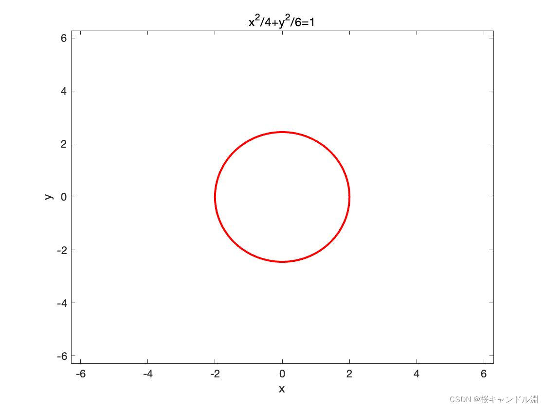

9. Use meshgrid Draw multiple functions

Use meshgrid Can make our x,y The numbers in realize one-to-one correspondence , use meshgrid It allows us to draw multiple curves at the same time

% Logarithmic function 
clear                                  % Clear variables 
xm=3;                                % The largest independent variable 
x=0.1:0.1:xm;                    % Independent variable vector 
a=[1/exp(1),0.5:0.5:2,exp(1),10];   % Base vector 
[A,X]=meshgrid(a,x);      % Base and independent variable matrix 
Y=log(X)./log(A);              % Logarithmic function matrix 
figure                                 % Create a graphics window 
plot(x,Y,'LineWidth',2)       % Draw a family of function curves 
title(' Family of logarithmic function curves ','FontSize',16)  % Add title 
xlabel('\itx','FontSize',16)           % Add abscissa 
ylabel('\ity','FontSize',16)           % Add ordinate 
grid on                                % Gridding 
legend([repmat('\ita\rm=',length(a),1),num2str(a')],4)% Complex legend 
hold on                                % Keep attributes 
plot(x,-log(x),'*',x,log(x),'+',x,log10(x),'x')% Redraw natural logarithm and common logarithm curve

10. Find the inverse function

Use y=finverse(y) That is to say y Become an inverse function of itself

syms x
y=x^2;
z=finverse(y);
z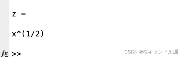

11. Find compound function

1. Use compose Find compound function

g=compose(f,g)

syms x
y=x^2;
g=sin(x);
z=compose(y,g);

syms x z
f=sin(x);
g=x^2;
compose(g,f)  % Returns the compound function g(f(y))
compose(g,f,x,z)  % The return argument is z

2. Use subs Find compound function

syms x z
f=sin(x);
g=x^2;
subs(g,f)  % Returns the compound function f(g(y))

12. Image with modulation curve

In front of some periodic functions , We can multiply some functions to plot our modulation curve , Let our function be constrained in two modulation curves . In the following code we use e^(-x) As our modulation curve

clc
clear
syms x
y=sin(pi*x)*exp(-x);
x=-5:0.01:5;
y=inline(y);
plot(x,y(x),x,exp(-x),x,-exp(-x),'LineWidth',2);

13. Automatically solve the equation

syms x a b c                      % Define symbolic variables 
x1=-2; y1=0; x2=0;y2=1; x3=1; y3=5;      %3 The horizontal of the point 、 Ordinate 
y=a*x^2+b*x+c;               % Quadratic sign function 
s1=subs(y,x,x1)-y1                     % The first 1 An algebraic equation 
s2=subs(y,x,x2)-y2                     % The first 2 An algebraic equation 
s3=subs(y,x,x3)-y3                     % The first 3 An algebraic equation 
[a,b,c]=solve(s1,s2,s3)