当前位置:网站首页>RFs self study notes (4): actual measurement model - the mixture of OK and CK, and then calculate the likelihood probability
RFs self study notes (4): actual measurement model - the mixture of OK and CK, and then calculate the likelihood probability
2022-07-28 19:14:00 【Learn something】
It involves the knowledge of joint probability distribution , Granulate the formula to facilitate computer calculation
The theoretical measurement model was introduced earlier O k O_k Ok And clutter model C k C_k Ck, Here is the actual measurement model Z k Z_k Zk, among , Z k = ( O k , C k ) Z_k=(O_k,C_k) Zk=(Ok,Ck), Express O k , C k O_k,C_k Ok,Ck Random arrangement means that the order is random . Think back to Bayesian filtering , What is the function of establishing measurement model ? Measure the likelihood probability of the model , Then we can use Bayesian formula to solve the posterior probability . So-called , Update step with Bayesian formula and measurement model .
Because the number of clutter is uncertain , This leads to the number of final measured values ∣ Z k ∣ |Z_k| ∣Zk∣ It's also uncertain , Set variables m = ∣ Z k ∣ m=|Z_k| m=∣Zk∣, Represents the number of element points contained in the measurement set . In addition, the concept of hypothesis needs to be introduced θ = { i > 0 i f − Z i − i s − a n − o b j e c t − d e t e c t i o n 0 i f − u n d e t e c t − o b j e c t \theta=\left\{\begin{matrix} i>0 &if- Z^i- is- an -object-detection\\ 0& if-undetect- object \end{matrix}\right. θ={ i>00if−Zi−is−an−object−detectionif−undetect−object for instance : Suppose now Z = [ 0.1 , 5.0 , 3.2 , 6.0 ] Z=[0.1,5.0,3.2,6.0] Z=[0.1,5.0,3.2,6.0] Yes 4 Measurements , this 4 All the measured values may be clutter, that is, no object is detected this time , It may also be that one of them is an object and the other three are clutter —— This is the assumption we started .
The first 0 The first assumption is θ = 0 \theta=0 θ=0 when : Indicates that no object has been detected , That is to say, this time Z Z Z The values in are all clutter . Then we can calculate the possibility of this situation according to the clutter model and the measurement model : If the detection probability of the sensor P D = 1 P^D=1 PD=1, That is to say, it is impossible to miss the inspection , So obviously this is the first 0 This assumption is very unreliable , The probability that this assumption can be established is 0. If the detection of the sensor is successful P D = 0.9 P^D=0.9 PD=0.9, That is to say, it may be missed , So this is 0 A hypothesis can happen , You need to calculate the number 0 The probability that a situation represented by a hypothesis can occur , At this time, after adding this assumption, this problem “ reduce to ” It's like this : In the known clutter model and measurement model, as well as the measured value this time Z Z Z after , The measured values this time are all clutter, that is, they all come from the clutter model , Find the probability of this happening ? First, it is judged that there is no object detected : 1 − P D 1-P^D 1−PD; Then the number of clutter conforms to Poisson distribution , Calculate the probability value corresponding to the number of clutter ; Finally, ask Z k i Z_k^i Zki It's all clutter , Find the corresponding probability value , Then you can get tired . Calculation formula : ( 1 − P D ) P o ( m ; λ c ) ∏ i = 1 m f c ( Z i ) = ( 1 − P D ) e − λ c m ! ∏ i = 1 m λ ( Z i ) = ( 1 − 0.9 ) e − 3 4 ! λ ( 0.1 ) λ ( 5.0 ) λ ( 3.2 ) λ ( 6.0 ) (1-P^D)Po(m;\lambda_c)\prod_{i=1}^{m}f_c(Z^i)=\\(1-P^D)\frac{e^{-\lambda_c}}{m!}\prod_{i=1}^{m}\lambda(Z^i)=\\(1-0.9)\frac{e^{-3}}{4!}\lambda(0.1)\lambda(5.0)\lambda(3.2)\lambda(6.0) (1−PD)Po(m;λc)i=1∏mfc(Zi)=(1−PD)m!e−λci=1∏mλ(Zi)=(1−0.9)4!e−3λ(0.1)λ(5.0)λ(3.2)λ(6.0) here , We take the average Poisson's ratio as 3, Z Z Z The number of elements in is obviously 4, The other is to bring Z k i Z_k^i Zki Into the intensity function . We can also determine an intensity function arbitrarily here f c ( c ) = { 1 4 c ∈ [ 3 , 7 ] 0 o t h e r s f_c(c)=\left\{\begin{matrix} \frac{1}{4} &c\in[3,7] \\ 0 &others \end{matrix}\right. fc(c)={ 410c∈[3,7]others and λ ( c ) = λ c f c ( c ) , \lambda(c)=\lambda_cf_c(c), λ(c)=λcfc(c), Then it can be evaluated : 0.1 ∗ e − 3 4 ! ∗ ( 3 / 4 ) 3 0.1*\frac{e^{-3}}{4!}*(3/4)^3 0.1∗4!e−3∗(3/4)3
Something doesn't feel right !!!—— This λ ( 0.1 ) \lambda(0.1) λ(0.1) What is the value of ? yes 0 still 1?( What is uniform distribution ?? Probability density and probability distribution should be able to distinguish !)
The first 1 The first assumption is θ = 1 \theta=1 θ=1 when : Express Z θ = Z 1 Z^{\theta}=Z^1 Zθ=Z1 It's an object , The other three are clutter . Obviously, this situation exists , We also need to calculate the probability of this happening . problem “ reduce to ”: In the known clutter model and measurement model, as well as the measured value this time Z Z Z after , Among the measured values this time Z θ = Z 1 Z^{\theta}=Z^1 Zθ=Z1 It is the object that comes from the measurement model , The rest are clutter, that is, they all come from the clutter model , Find the probability of this happening ? The calculated probability is : P D P o ( m − 1 ; λ c ) 1 m g k ( z θ ∣ x ) ∏ i = 1 m f c ( z i ) f c ( z θ ) = P D g k ( z θ ∣ x ) λ ( z θ ) e − λ c m ! ∏ i = 1 m λ ( z i ) = 0.9 ∗ g k ( z 1 ∣ x ) λ ( z 1 ) e − 3 4 ! λ ( z 1 ) λ ( z 2 ) λ ( z 3 ) λ ( z 4 ) P^DPo(m-1;\lambda_c)\frac{1}{m}g_k(z^{\theta}|x)\frac{\prod_{i=1}^{m}f_c(z^i)}{f_c(z^{\theta})}\\=P^D\frac{g_k(z^{\theta}|x)}{\lambda(z^{\theta})}\frac{e^{-\lambda_c}}{m!}\prod_{i=1}^{m}\lambda(z^i)\\=0.9*\frac{g_k(z^{1}|x)}{\lambda(z^{1})}\frac{e^{-3}}{4!}\lambda(z^1)\lambda(z^2)\lambda(z^3)\lambda(z^4) PDPo(m−1;λc)m1gk(zθ∣x)fc(zθ)∏i=1mfc(zi)=PDλ(zθ)gk(zθ∣x)m!e−λci=1∏mλ(zi)=0.9∗λ(z1)gk(z1∣x)4!e−3λ(z1)λ(z2)λ(z3)λ(z4) there g k ( ) g_k() gk() Is the probability distribution of the theoretical measurement model , Reflect the measurement accuracy of the sensor , When simplifying problems , It can be said that g k ( ) g_k() gk() It's a normal distribution , The reference quantity is x x x.
The first 2 The first assumption is θ = 2 \theta=2 θ=2 when : Express Z θ = Z 2 Z^{\theta}=Z^2 Zθ=Z2 It's an object , The other three are clutter .
The first 3 The first assumption is θ = 3 \theta=3 θ=3 when : Express Z θ = Z 3 Z^{\theta}=Z^3 Zθ=Z3 It's an object , The other three are clutter .
The first 4 The first assumption is θ = 4 \theta=4 θ=4 when : Express Z θ = Z 4 Z^{\theta}=Z^4 Zθ=Z4 It's an object , The other three are clutter .
common 5 A hypothesis , It covers all possible situations
Put this 5 The probabilities of each case can be added ?? The final result is a multimodal distribution ??
Derivation and calculation of likelihood probability
m m m Express Z Z Z The number of elements in , θ \theta θ Indicates the assumptions made
p ( Z ∣ X ) = p ( Z , m ∣ X ) = ∑ θ = 0 m p ( Z , m , θ ∣ X ) p(Z|X)=p(Z,m|X)=\sum_{\theta=0}^{m}p(Z,m,\theta|X) p(Z∣X)=p(Z,m∣X)=θ=0∑mp(Z,m,θ∣X) because Z Z Z After setting , m m m Then it was decided that m m m It's actually contained in Z Z Z Information in , So there can be p ( Z ∣ X ) = p ( Z , m ∣ X ) p(Z|X)=p(Z,m|X) p(Z∣X)=p(Z,m∣X), here p ( Z , m ∣ X ) p(Z,m|X) p(Z,m∣X) It's about ( Z , m ) (Z,m) (Z,m) Two dimensional joint probability distribution , But these two variables are not independent , It's about containing relationships . and p ( Z , m , θ ∣ X ) p(Z,m,\theta|X) p(Z,m,θ∣X) It's about ( Z , m , θ ) (Z,m,\theta) (Z,m,θ) Three dimensional joint probability distribution , here Z Z Z and θ \theta θ Then there is no containment relationship , It is closer to the general two-dimensional joint distribution . And yes θ \theta θ The sum of variables is equal to θ \theta θ Find integral , Is equivalent to θ \theta θ It's gone , The result is about Z Z Z Edge density of .
 Supplement the formula of joint probability distribution

p(A,B) = p(B|A)p(A)

p(a,b|c) = p(a,b,c)/p(c) = [p(a,b,c)/p(b,c)] * [p(b,c)/p(c)]
         = p(a|b,c)p(b|c)
set up A A A event : Z Z Z; B B B event : m m m; C C C event : θ \theta θ; D D D event : X X X; among B B B Events are contained in A A A Incident
be p ( A , B , C ∣ D ) = p ( A , B , C , D ) p ( D ) p(A,B,C|D)=\frac{p(A,B,C,D)}{p(D)} p(A,B,C∣D)=p(D)p(A,B,C,D) because p ( A ∣ B , C , D ) = p ( A , B , C , D ) p ( B , C , D ) p(A|B,C,D)=\frac{p(A,B,C,D)}{p(B,C,D)} p(A∣B,C,D)=p(B,C,D)p(A,B,C,D) Bring it into the above formula p ( A , B , C ∣ D ) = p ( A , B , C , D ) p ( D ) = p ( A ∣ B , C , D ) p ( B , C , D ) p ( D ) = p ( A ∣ B , C , D ) p ( B , C ∣ D ) p(A,B,C|D)=\frac{p(A,B,C,D)}{p(D)}\\=\frac{p(A|B,C,D)p(B,C,D)}{p(D)}\\=p(A|B,C,D)p(B,C|D) p(A,B,C∣D)=p(D)p(A,B,C,D)=p(D)p(A∣B,C,D)p(B,C,D)=p(A∣B,C,D)p(B,C∣D) Or get p ( Z ∣ X ) = ∑ θ = 0 m p ( Z ∣ m , θ , X ) p ( θ , m ∣ X ) p(Z|X)=\sum_{\theta=0}^{m}p(Z|m,\theta,X)p(\theta,m|X) p(Z∣X)=θ=0∑mp(Z∣m,θ,X)p(θ,m∣X) Now briefly explain the meaning of each item
p ( Z ∣ m , θ , X ) p(Z|m,\theta,X) p(Z∣m,θ,X): Number of known elements m m m、 Specific to a certain assumption θ \theta θ、 Truth value X X X when , Find out how much probability the sensor will measure Z Z Z—— With θ = 1 \theta=1 θ=1 For example : It is measured as z 1 z^1 z1 It's an object and comes from a theoretical measurement model , Other z 2 , z 3 , z 4 z^2,z^3,z^4 z2,z3,z4 They are all clutter points and come from the clutter model . This is under hypothetical conditions ( Adding this assumption simplifies the original problem ) Ask again Z Z Z, It represents a simplified problem .
p ( m , θ ∣ X ) p(m,\theta|X) p(m,θ∣X): according to X X X determine m , θ m,\theta m,θ Value —— That is, how much probability there will be m m m Element and is the θ \theta θ A hypothesis , Similar to the reliability of assumptions . according to X X X To infer the number of measurement results and which measurement value will be an object , The reliability of this inference .
Understanding the derivation of this part and the significance of these two terms can better understand the actual measurement model , So as to obtain the actual likelihood probability .
Next, calculate these two terms respectively , Then multiply it to find the , Finally, add up to get the final result .
When θ = 0 \theta=0 θ=0 when , Indicates that the object has not been detected , m m m Clutter detection .
At this time , p ( m , θ ∣ X ) p(m,\theta|X) p(m,θ∣X) The corresponding inference is : There are 0 0 0 An object , Yes m m m A clutter . The probability of the former is 1 − P D 1-P^D 1−PD, The probability of the latter is P o ( m ; λ c ) Po(m;\lambda_c) Po(m;λc). This item is mainly used to determine assumptions —— That is to distinguish which item is an object , Which items are clutter , So it's actually about the determination of the number . Therefore, it just corresponds to the Bernoulli detection part of the measurement model and the Poisson distribution part of the clutter model , These two parts are related to the number . The distribution characteristics of a specific point are g k ( ) g_k() gk() and f c ( ) f_c() fc(), This is a p ( Z ∣ m , θ , X ) p(Z|m,\theta,X) p(Z∣m,θ,X) This one is responsible . Then the formula is : p ( m , θ = 0 ∣ X ) = ( 1 − P D ) P o ( m ; λ c ) p(m,\theta=0|X)=(1-P^D)Po(m;\lambda_c) p(m,θ=0∣X)=(1−PD)Po(m;λc)
and p ( Z ∣ m , θ , X ) p(Z|m,\theta,X) p(Z∣m,θ,X): When Z Z Z The elements in it are all clutter m m m A clutter , Find the probability of this happening —— Simplified problems after adding assumptions . The formula is : p ( Z ∣ m , θ = 0 , X ) = ∏ i = 1 m f c ( z i ) p(Z|m,\theta=0,X)=\prod_{i=1}^{m}f_c(z^i) p(Z∣m,θ=0,X)=i=1∏mfc(zi)
When θ = 1 \theta=1 θ=1 when , Express z 1 z^1 z1 It's an object , other m − 1 m-1 m−1 All measurement points are clutter .
here , p ( m , θ = 1 ∣ X ) p(m,\theta=1|X) p(m,θ=1∣X) The corresponding inference is : There are 1 1 1 An object is z 1 z^1 z1, Yes m − 1 m-1 m−1 A clutter . The probability of the former is P D P^D PD That is, the object is successfully detected , The probability of the latter is P o ( m − 1 ; λ c ) 1 m Po(m-1;\lambda_c)\frac{1}{m} Po(m−1;λc)m1—— Poisson distribution indicates that there are m − 1 m-1 m−1 A clutter , but 1 m \frac{1}{m} m1 What does it mean ? Express P ( θ = 1 ) = 1 / m ? P(\theta=1)=1/m? P(θ=1)=1/m? Calculation formula : p ( m , θ = 1 ∣ X ) = P D P o ( m − 1 ; λ c ) 1 m p(m,\theta=1|X)=P^DPo(m-1;\lambda_c)\frac{1}{m} p(m,θ=1∣X)=PDPo(m−1;λc)m1
and p ( Z ∣ m , θ = 1 , X ) p(Z|m,\theta=1,X) p(Z∣m,θ=1,X): When Z Z Z There are only z 1 z^1 z1 It's an object , Other elements are clutter m − 1 m-1 m−1 A clutter , Find the probability of this happening —— Simplified problems after adding assumptions . Its calculation formula : p ( Z ∣ m , θ = 1 , X ) = g k ( z 1 ∣ x ) ∏ i = 1 m f c ( z i ) f c ( z 1 ) p(Z|m,\theta=1,X)=g_k(z^1|x)\frac{\prod_{i=1}^{m}f_c(z^i)}{f_c(z^1)} p(Z∣m,θ=1,X)=gk(z1∣x)fc(z1)∏i=1mfc(zi) Why... Here z z z As a result of g k ( ) g_k() gk() The argument to the function , Should not be o o o Do you ?—— because z z z By ( o , c ) (o,c) (o,c) The result of mixed arrangement , So naturally there is one z j z^j zj Namely o o o, So this z j z^j zj Just follow this o o o Conform to the theoretical measurement model g k ( ) g_k() gk() 了 . The rest z z z The element is determined to be a clutter point , From the clutter model , Nature is in line with f c ( ) f_c() fc() 了 .
Empathy , The calculation formula of other assumptions can be deduced, namely θ ∈ ( 1 , 2 , 3 , . . . , m ) \theta\in (1,2,3,...,m) θ∈(1,2,3,...,m), Then add up the results corresponding to all assumptions to get p ( z ∣ x ) p(z|x) p(z∣x), Expression for p ( z ∣ x ) = ∑ θ = 0 m p ( z , m , θ ∣ x ) = [ ( 1 − P D ) + P D ∑ θ = 1 m g k ( z θ ∣ x ) λ ( z θ ) ] e − λ c m ! ∏ i = 1 m λ ( z i ) p(z|x)=\sum_{\theta=0}^{m}p(z,m,\theta|x)\\=[(1-P^D)+P^D\sum_{\theta=1}^{m}\frac{g_k(z^{\theta}|x)}{\lambda(z^{\theta})}]\frac{e^{-\lambda_c}}{m!}\prod_{i=1}^{m}\lambda(z^i) p(z∣x)=θ=0∑mp(z,m,θ∣x)=[(1−PD)+PDθ=1∑mλ(zθ)gk(zθ∣x)]m!e−λci=1∏mλ(zi) This is the calculation formula of likelihood probability obtained from the actual measurement model , Later, it can be used in Bayesian formula , To complete the update step .
边栏推荐
- [R language - basic drawing]
- 湖上建仓全解析:如何打造湖仓一体数据平台 | DEEPNOVA技术荟系列公开课第四期
- The difference between --save Dev and --save in NPM
- How to solve the problem that easycvr device cannot be online again after offline?
- How to break through the bottleneck of professional development for software testing engineers
- Pytorch GPU yolov5 reports an error
- How to write a JMeter script common to the test team
- From Bayesian filter to Kalman filter (zero)
- Special Lecture 6 tree DP learning experience (long-term update)
- Why did wechat change from "small and beautiful" to "big and fat" when it expanded 575 times in 11 years?
猜你喜欢

配置教程:新版本EasyCVR(v2.5.0)组织结构如何级联到上级平台?
Efficiency comparison of JS array splicing push() concat() methods

QT user defined control user guide (flying Qingyun)

Is software testing really as good as online?

PyG搭建异质图注意力网络HAN实现DBLP节点预测
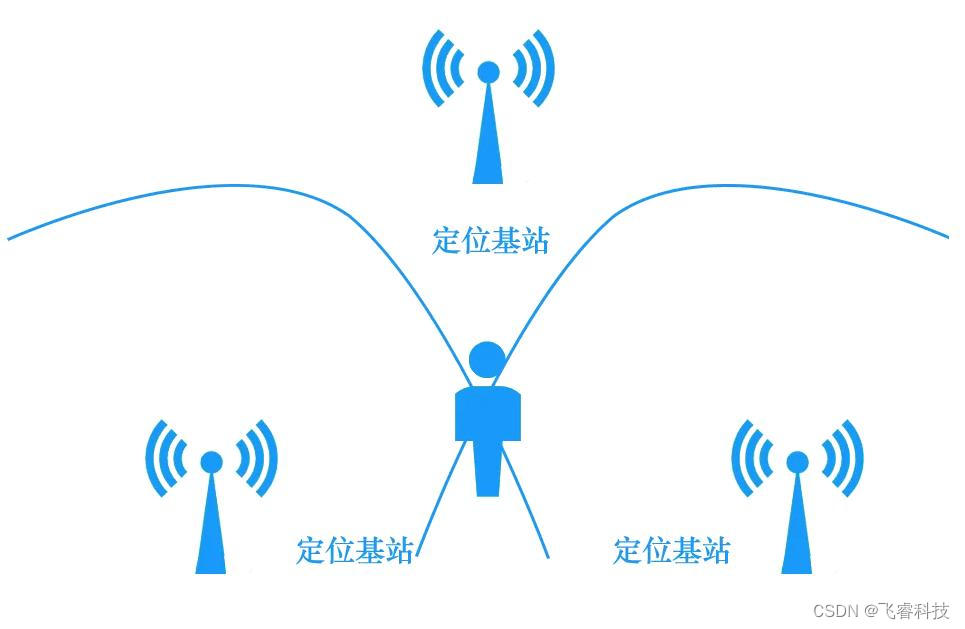
uwb模块实现人员精确定位,超宽带脉冲技术方案,实时厘米级定位应用

AI 改变千行万业,开发者如何投身 AI 语音新“声”态
![[R language - basic drawing]](/img/1e/aebf1cbe02c4574671bac6dc2c9171.png)
[R language - basic drawing]

Youqilin system installation beyondcomare

BM16 删除有序链表中重复的元素-II
随机推荐
直播平台软件开发,js实现按照首字母排序
Applet applet jump to official account page
Win11电脑摄像头打开看不见,显示黑屏如何解决?
2022年牛客多校第2场 J . Link with Arithmetic Progression (三分+枚举)
优麒麟系统安装BeyondComare
Is two months of software testing training reliable?
[R language - basic drawing]
Can the training software test be employed
Xiaobai must see the development route of software testing
QT with line encoding output cout
The login interface of modern personal blog system modstartblog v5.4.0 has been revised and the contact information has been added
Getting started with QT & OpenGL
GC garbage collector details
QT function optimization: QT 3D gallery
uwb模块实现人员精确定位,超宽带脉冲技术方案,实时厘米级定位应用
湖上建仓全解析:如何打造湖仓一体数据平台 | DEEPNOVA技术荟系列公开课第四期
Is it useful to learn software testing?
If you want to learn software testing, where can you learn zero foundation?
Easynlp Chinese text and image generation model takes you to become an artist in seconds
BM14 链表的奇偶重排