Chapter 2 of machine learning [series] logistic regression model

machine learning 【 series 】 The second chapter is the logistic regression model

Chapter two Logistic regression model

---

---

Preface

This chapter mainly explains the classic logistic regression model in machine learning , Including the algorithm principle and programming implementation of logistic regression , And through a classic case of logistic regression ------ Customer churn early warning model , To consolidate what we have learned , Finally, it will explain the common model evaluation methods for classification models in machine learning .

The linear regression model learned in the previous chapter is a regression model , It predicts continuous variables , Such as the predicted income range , Customer value, etc . If you want to predict discrete variables , Use the classification model . The difference between the classification model and the regression model is that the variables predicted by the classification model are discontinuous , But some discrete differences , for example , The most common binary model can predict whether a person will default 、 Whether there will be a loss of customers 、 Is the tumor benign or malignant . The logistic regression model to be studied in this chapter has “ Return to ” Two words , But it is a classification model in essence .

---

One 、 Algorithm principle of logistic regression model

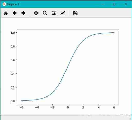
The following code can be used to draw Sigmoid The image of the function ：

import matplotlib.pyplot as plt
import numpy as np

x = np.linspace(-6,6)  #  adopt linespace() Function generation -6——6 Equal difference sequence of , Default 50 Number 
y = 1.0/(1.0+np.exp(-x))
# Sigmod Function calculation formula ,exp() Is a natural number constant e The exponential function at the bottom 
plt.plot(x,y)
plt.show()

The essence of logistic regression model is to predict the probability of each classification , With probability , So we can sort it out . For the problem of two categories , For example, in a model that predicts whether a customer will default , If the predicted probability of default is P by 70%, Then the probability of default is 30%, The probability of default is greater than the probability of non default , At this point, it can be considered that the customer will default . For multi classification problems , Logistic regression models predict the probability of belonging to each category （ The sum of the probabilities is 1）, Then according to which probability is the greatest , Decide which category you belong to .
After knowing the basic principle of logistic regression model , In the actual model building , Is to find the appropriate coefficient ki And intercept terms k0, Make the probability of prediction more accurate , In mathematics, maximum likelihood estimation is used to determine appropriate coefficients ki And intercept terms k0.

Students who want to know more about the principle of its mathematical algorithm can search for information , It's not going to unfold here .

Two 、 Code implementation of logistic regression model

1. Code implementation of logistic regression model

X = [[1, 0], [5, 1], [6, 4], [4, 2], [3, 2]]
y = [0, 1, 1, 0, 0]

from sklearn.linear_model import LogisticRegression
model = LogisticRegression()
model.fit(X, y)  

print(model.predict([[2,2]]))
print(model.predict([[1,1], [2,2], [5, 5]]))
print(model.predict([[1, 0], [5, 1], [6, 4], [4, 2], [3, 2]]))  
#  Because the multiple data and X It's the same , So it can also be written directly as model.predict(X)

--> The output is ：
[0]
[0 0 1]
[0 1 1 1 0]

2. In depth understanding of logistic regression models

The code is as follows （ Example ）：

import pandas as pd
a = pd.DataFrame(y_pred_proba, columns=[' Classified as 0 Probability ', ' Classified as 1 Probability '])  # 2.2.1  adopt numpy Array creation DataFrame
print(a)
print(model.coef_)  #  Printout factor k1,k2
print(model.intercept_) # Printout intercept items k0

3. Supplementary information ： Using logistic regression model to deal with multi classification problems

X = [[1, 0], [5, 1], [6, 4], [4, 2], [3, 2]]
y = [-1, 0, 1, 1, 1]

from sklearn.linear_model import LogisticRegression
model = LogisticRegression()
model.fit(X, y)

print(model.predict([[0, 0]]))

model.predict(X)
print(model.predict_proba([[0, 0]]))

--> The output is ：
[-1]
[[0.40456707 0.27958903 0.3158439 ]]

3、 ... and 、 Case actual combat ： Customer churn early warning model

1. Case background

If a client no longer trades through a securities firm , That is, the customer lost , Then the securities company loses a source of income , therefore , Securities companies will build a set of customer churn early warning model to predict whether customers will be lost , And take corresponding recovery measures for customers with high loss probability , Because usually , The cost of acquiring new customers is much higher than the cost of retaining existing customers .

2. Data reading and variable partition

# 1. Reading data 
df = pd.read_excel(" Stock customer churn .xlsx")
# print(df.head())

# 2. Divide characteristic variables and target variables 
X = df.drop(columns=' Is it lost ')
y = df[" Is it lost "]

3. Model construction and use

1. Divide the training set and the test set

from sklearn.model_selection import train_test_split
X_train,X_test,y_train,y_test = train_test_split(X,y,test_size=0.2,random_state=1)

2. Model structures,

from sklearn.linear_model import LogisticRegression
model = LogisticRegression()
model.fit(X_train,y_train)  #  The input parameter is the number of training sets obtained in the previous step X_train,y_train

3 Model USES 1： Forecast data results

y_pred = model.predict(X_test)

a = pd.DataFrame() #  Create an empty DataFrame
a[" Predictive value "] = list(y_pred)
a[" actual value "] = list(y_test)
# print(a.head())

#  View the prediction accuracy of all test set data 
#  Method 1 :
from sklearn.metrics import accuracy_score
score = accuracy_score(y_pred,y_test)
# print(score)
#  Method 2 ：
# print(model.score(X_test,y_test))

4. Model USES 2： Prediction probability

y_pred_prba = model.predict_log_proba(X_test)
a = pd.DataFrame(y_pred_prba,columns=[" No loss probability "," Loss probability "])
print(a.head())

5. Obtain the logistic regression coefficient

print(model.coef_)
print(model.intercept_)

--> The output is ：
[[ 2.38800779e-05  8.05683618e-03  1.03327747e-02 -2.52102650e-03 -1.11180522e-04]]
[-1.41822666e-06]

Four 、 Model evaluation method ：ROC Curve and KS curve

1.ROC Basic principle of curve

（ Explain according to the above case ） among

1. 986 by True Positive(TP) To affirm correctly
2. 93 by False Negative(FN) Omission of
3. 194 by False Positive(FP) A false report
4. 154 by True Negative(TN) To deny correctly

shooting （TPR）= Customers predicted to be lost and actually lost / Actual lost customers
False alarm rate （FPR）= Customers predicted to be lost but not actually lost / Customers who have not actually lost

An excellent customer churn early warning model , shooting （TPR） It should be as high as possible , That is, we can try to find out potential lost customers , At the same time, the false alarm rate （RPR） It should be as low as possible , That is, don't misjudge non lost customers as lost customers .

2. Confusion matrix Python Code implementation

from sklearn.metrics import confusion_matrix
m = confusion_matrix(y_test,y_pred)
a = pd.DataFrame(m,index=["0( Actually, there is no loss )","1( Predicted loss )"],columns=["0( No loss of prediction )","1( Predicted loss )"])
print(a)

from sklearn.metrics import classification_report
print(classification_report(y_test,y_pred))  #  Pass in predicted and actual values 

3. Case actual combat ： use ROC Curve assessment customer churn warning

Model

from sklearn.metrics import roc_curve
fpr,tpr,thres = roc_curve(y_test,y_pred_proba[:,1])
a = pd.DataFrame()
a[" threshold "] = list(thres)
a[" False alarm rate "] = list(fpr)
a[" shooting "] = list(tpr)

roc_curve() Function passes in the target variable of the test set y_test And predict the loss probability y_pred_proba[:,1], Calculate the hit rate and false alarm rate under different thresholds . because roc_curve() The function returns a 3 Tuples of elements , Among them, the default is no 1 Elements are false alarm rate , The first 2 The first element is the hit rate , The first 3 Elements are threshold , So here we assign these three to variables fpr（ False alarm rate ）、tpr（ shooting ）、thres（ threshold ）.

import matplotlib.pyplot as plt
plt.plot(fpr,tpr)
plt.title("ROC")
plt.xlabel("FPR")
plt.ylabel("TPR")
plt.show()

4.KS Basic principle of curve

KS Curves and ROC The curves are essentially the same , Also focus on hit rate （TPR） And false alarm rate （FPR）, Hope the hit rate （TPR） As high as possible , That is to find out potential lost customers , At the same time, we also hope that the false alarm rate （FPR） As low as possible , That is, don't misjudge non lost customers as lost customers .
KS The value is KS The peak of the curve
In general , We want the model to have a larger KS value , Because the bigger KS Value indicates that the model has strong distinguishing ability , Of different value ranges KS The meaning of the value is as follows ：

• KS Less than 0.2, It is generally believed that the discrimination ability of the model is weak ;
• KS The value is in the range [0.2,0.3] Within the interval , The model has some distinguishing ability ;
• KS The value is in the range [0.3,0.5] Within the interval , The model has strong distinguishing ability .

but KS The bigger the value, the better , If KS Greater than 0.75, It often indicates that the model is abnormal . In business practice ,KS Value in [0.2,0.3] It's pretty good in the range .

5. Case actual combat ： use KS Curve evaluation customer churn early warning model

from sklearn.metrics import roc_curve
fpr,tpr,thres = roc_curve(y_test,y_pred_proba[:,1])
a = pd.DataFrame()
a[" threshold "] = list(thres)
a[" False alarm rate "] = list(fpr)
a[" shooting "] = list(tpr)


#  Because the threshold in the first row of the table is greater than 1, meaningless , Will result in unsightly graphics , So the first row is removed by slicing ,
 among thres[1:],tpr[1:],fpr[1:] Both represent drawing from the second element .
plt.plot(thres[1:],tpr[1:])
plt.plot(thres[1:],fpr[1:])
plt.plot(thres[1:],tpr[1:]-fpr[1:])
plt.xlabel("threshold")
plt.legend(["tpr","fpr","tpr-fpr"])
plt.gca().invert_xaxis()
#  First use gca() Function to get information about the coordinate axis , In use invert_xaxis() Function inversion x Axis 
plt.show()


#  Quickly find KS value 
print(max(tpr-fpr))
---> The output is ：
0.4754081488944501

---

summary

Reference books ：《Python Big data analysis and machine learning business case practice 》