当前位置:网站首页>Formatting the generalization forgetting trade off in continuous learning
Formatting the generalization forgetting trade off in continuous learning
2022-06-12 07:17:00 【Programmer long】
The address of the paper is here
One . Introduce
In continuous learning , Learn sequential observed tasks by gradually adapting to a model . It has two main objectives : Keep long-term memory and keep learning new knowledge . And that is stability - The dilemma of plasticity , And continuous learning is trying to find a balance between the two .
Conventional CL Methods either minimize catastrophic forgetting , Or improve rapid generalization , Without simultaneous consideration . Common can be divided into three categories :(1) Dynamic network structure ,(2) Regularization approach ,(3) Memory replay is the way of scene reproduction . The solution to the generalization problem includes the way to express learning ( For example, meta learning ).
These traditional CL The method only minimizes a loss function , However, the trade-offs in their re optimization settings are not explicitly considered . The first person to consider this work is meta-experience replay(MER) In the algorithm, , Among them, forget - Generalization is proposed as a way of gradient alignment . But in MER in , The balance of forgetting generalization is achieved by several super parameters . therefore , There are two challenges , One is the lack of universal theory tools to study the existence and stability of an equilibrium point . The second is the lack of Pan system method to achieve this balance point . Therefore, this paper is to improve this .
The author describes a framework , In this framework , First of all, will CL The problem is defined as a sequential decision problem , And seek to minimize the total cost function of the whole model life cycle . At any time , If future missions are not available , The calculation of cost function becomes very difficult . To solve this problem , utilize Bellman The optimality principle of , Yes CL Re model the problem , To simulate the catastrophic forgetting cost of previous tasks and the generalization cost of new tasks . And then make improvement according to this , A balanced continuous learning algorithm is proposed (BCL).
Two . Problem definition
In this paper R , N \mathbb{R,N} R,N Represents a real number field and a positive integer field . ∥ . ∥ \parallel . \parallel ∥.∥ Denotes the universal number of a matrix . All in all [ 0 , K ] , K ∈ N [0,K],K\in \mathbb{N} [0,K],K∈N A mission . The model is g ( . ) g(.) g(.), Accept θ k \theta_k θk Parameters predict the data . A task ( Suppose it's the k A mission ), Expressed as Q k = { X k , l k } \mathcal{Q}_k = \{\mathcal{X_k,l_k}\} Qk={ Xk,lk}, among l For the corresponding loss . The representation of the parameter sequence is u k : K = { θ τ ∈ Ω θ , k ≤ τ ≤ K } u_{k:K}=\{\theta_{\tau}\in\Omega_{\theta},k\le\tau\le K\} uk:K={ θτ∈Ωθ,k≤τ≤K}, among , Ω θ \Omega_\theta Ωθ Represents a compact set .* Expressed as the optimal value ( for example θ ∗ \theta^* θ∗).
Here the author gives a diagram to describe continuous learning :
In order to make continuous learning concrete , Here a consumption is defined (cost): Forgotten by disaster cost And generalization . This cost In every task k There's always : J k ( θ k ) = γ k ℓ k + ∑ τ = 0 k − 1 γ τ ℓ τ J_k(\theta_k) = \gamma_k\ell_k+\sum^{k-1}_{\tau=0}\gamma_\tau \ell_\tau Jk(θk)=γkℓk+∑τ=0k−1γτℓτ. there ℓ τ \ell_\tau ℓτ Be calculated in the task Q τ \mathcal{Q}\tau Qτ, Describe the contribution of this task to the sum . In order to solve the problem in k The problem at this time on the task , We need to find θ k \theta_k θk bring J k ( θ k ) J_k(\theta_k) Jk(θk) Minimum . So for the whole task sequence , We need to keep it to a minimum . Therefore, the whole optimization problem of continuous learning is accumulation cost: V k ( u k : K ) = ∑ τ = k K β τ J τ ( θ τ ) V_k(u_{k:K})=\sum^K_{\tau=k}\beta_\tau J_\tau(\theta_\tau) Vk(uk:K)=∑τ=kKβτJτ(θτ), Make it the smallest :
V k ( ∗ ) = min u k : K V k ( u k : K ) (1) V^{(*)}_k=\min _{u_{k:K}}V_k(u_{k:K}) \tag{1} Vk(∗)=uk:KminVk(uk:K)(1)
In this formula , There are two parameters that determine the contribution of the task : γ τ \gamma_\tau γτ, I didn't think about the contribution of the task in the past . β τ \beta_\tau βτ, Contribution to future missions . To solve this problem ,(1) Must be continuously differentiable . Then the author proves that it is differentiable in the case that infinite tasks cannot be guaranteed , At the same time, it is also said that a with infinite memory CL The problem is np problem ,CL Can't provide perfect performance on a large number of tasks , And the task must have a priority . So it would be wrong just to naively reduce this loss , And because the previous data is not visible , It is not possible to evaluate previously processed tasks .
3、 ... and . Continuous learning of dynamic programming
Firstly, the representation of dynamic programming is introduced ( That is, the optimal cost for k The performance of the ):
∇ k ( V k ( ∗ ) ) = − min θ k ∈ Ω θ [ β k J k ( θ k ) + ( < ∇ θ k V k ( ∗ ) , Δ θ k > + < ∇ x k V k ( ∗ ) , Δ x k > ) ] (2) \nabla_k(V_k^{(*)})=-\min_{\theta_{k}\in\Omega_\theta}[\beta_k J_k(\theta_k)+(<\nabla_{\theta_k}V_k^{(*)},\Delta\theta_k>+<\nabla_{x_k}V_k^{(*)},\Delta x_k>)] \tag{2} ∇k(Vk(∗))=−θk∈Ωθmin[βkJk(θk)+(<∇θkVk(∗),Δθk>+<∇xkVk(∗),Δxk>)](2)
(2) The derivation of is omitted here , If you are interested, you can read the original . In the formula ∇ k ( V k ( ∗ ) ) \nabla_k(V_k^{(*)}) ∇k(Vk(∗)) Express V k ( ∗ ) V_k^{(*)} Vk(∗) All disturbances in . in other words , When it equals 0 Explain the new task k Will not affect our current solution , let me put it another way , The optimal solution for the previous task is also the optimal solution for the new task . So the smaller the disturbance , The better the performance of the model for all tasks , So the goal becomes : Minimize all disturbances . stay (2) in , This disturbance has three parts : Cost distribution for previous tasks plus tasks k: J k ( θ k ) J_k(\theta_k) Jk(θk), Parameter changes < ∇ θ k V k ( ∗ ) , Δ θ k > <\nabla_{\theta_k}V_k^{(*)},\Delta\theta_k> <∇θkVk(∗),Δθk>, And the introduction of new tasks ( Data sets ) And lead to the change of optimal cost < ∇ x k V k ( ∗ ) , Δ x k > <\nabla_{x_k}V_k^{(*)},\Delta x_k> <∇xkVk(∗),Δxk>.
Optimize (2) The task is to find the solution of continuous learning . We use it H ( Δ x k , θ k ) = β k J k ( θ k ) + ( < ∇ θ k V k ( ∗ ) , Δ θ k > + < ∇ x k V k ( ∗ ) , Δ x k > ) H(\Delta x_k,\theta_k) = \beta_k J_k(\theta_k)+(<\nabla_{\theta_k}V_k^{(*)},\Delta\theta_k>+<\nabla_{x_k}V_k^{(*)},\Delta x_k>) H(Δxk,θk)=βkJk(θk)+(<∇θkVk(∗),Δθk>+<∇xkVk(∗),Δxk>). That is, optimize H ( Δ x k , θ k ) H(\Delta x_k,\theta_k) H(Δxk,θk) It means to minimize the interference caused by new tasks .
Next , We must balance generalization and forgetting for each task k. When the model successfully adapts to the new task , It shows generalization . The degree of generalization depends on the difference between the previous task and the new task . The greater the difference between the two follow-up tasks , The more general the model must be . therefore , Worst case differences suggest maximum generalization . However , Larger differences increase forgetfulness , The worst-case difference produces the greatest forgetfulness . At the same time make (2) The value of the third term in is the largest , Maximum generalization can be obtained , therefore Δ x k \Delta x_k Δxk Quantifying changes in subsequent tasks . However Δ x k = x k + 1 − x k \Delta x_k=x_{k+1}-x_k Δxk=xk+1−xk, We don't know x k + 1 x_{k+1} xk+1 When the first k A task . So use update Δ x k \Delta x_k Δxk The gradient rises to estimate the difference in the worst case . Next , Update by iterating using gradient descent θ k \theta_k θk To minimize maximum generalization forgetting .
Next , To describe the above problem . Superscript i It means the first one k Iteration of task No i round .
stay (3) in , Try to find a group ( Δ x k ( ∗ ) , θ k ( ∗ ) ) (\Delta x_k^{(*)},\theta_k^{(*)}) (Δxk(∗),θk(∗)), among Δ x k ( ∗ ) \Delta x_k^{(*)} Δxk(∗) send H Maximize , and θ k ( ∗ ) \theta_k^{(*)} θk(∗) send H To minimize the ( This is what the author said above , Two player, Find the balance ). ( Δ x k ( ∗ ) , θ k ( ∗ ) ) (\Delta x_k^{(*)},\theta_k^{(*)}) (Δxk(∗),θk(∗)) For our solution , To meet the following conditions :
H ( Δ x k ( ∗ ) , θ k ( i ) ) ≥ H ( Δ x k ( ∗ ) , θ k ( ∗ ) ) ≥ H ( Δ x k ( i ) , θ k ( ∗ ) ) (4) H(\Delta x_k^{(*)},\theta_k^{(i)})\ge H(\Delta x_k^{(*)},\theta_k^{(*)}) \ge H(\Delta x_k^{(i)},\theta_k^{(*)}) \tag{4} H(Δxk(∗),θk(i))≥H(Δxk(∗),θk(∗))≥H(Δxk(i),θk(∗))(4)
3.1 The theoretical analysis
Now the goal is how to find the point we want , To achieve balance .
The above figure briefly describes the author's thinking . First, fix it at first θ \theta θ, Construct a neighborhood M k = θ k ( . ) ∈ Ω x } \mathcal{M}_k = \theta_k^{(.)}\in\Omega_x\} Mk=θk(.)∈Ωx}, And then to Δ x k ( i ) \Delta x_k^{(i)} Δxk(i), Find a local maximum in this interval by using the gradient rise . Next , Lock what we found Δ x k ( . ) \Delta x_k^{(.)} Δxk(.). Update according to gradient descent . Here the author proves that in N k = { Ω θ , Δ x k ( . ) } \mathcal{N}_k=\{\Omega_\theta,\Delta x_k^{(.)}\} Nk={ Ωθ,Δxk(.)} In this area ,H Is the minimum , At the same time, it converges to this region . Finally, in the above two areas , There is at least one equilibrium point here .
3.2 Balanced continuous learning (BCN)
Based on this , Let's change H ( Δ x k ( i ) , θ k ( i ) ) ≈ β k J k ( θ k ( i ) ) + ( J k ( θ k ( i + ζ ) ) − J k ( θ k ( i ) ) ) + ( J k + ζ ( θ k ( i ) ) − J k ( θ k ( i ) ) ) H(\Delta x_k^{(i)},\theta^{(i)}_k)\approx \beta_k J_k(\theta_k^{(i)})+(J_k(\theta_k^{(i+\zeta)}) - J_k(\theta_k^{(i)}) )+(J_{k+\zeta}(\theta_k^{(i)}) -J_k(\theta_{k}^{(i)}) ) H(Δxk(i),θk(i))≈βkJk(θk(i))+(Jk(θk(i+ζ))−Jk(θk(i)))+(Jk+ζ(θk(i))−Jk(θk(i))). among J k + ζ J_{k+\zeta} Jk+ζ It's about updating player 1, θ k ( i + ζ ) \theta_k^{(i+\zeta)} θk(i+ζ) It's an update player2.
Two of them player Use the above 5 Select and update . The specific algorithm is shown in the figure below :
among D N ( k ) \mathcal{D}_N(k) DN(k) This is a new task , D P ( k ) \mathcal{D}_P(k) DP(k) Indicates that samples are taken from past tasks . For each of these batch b N ∈ D N ( k ) b_N\in \mathcal{D}_N(k) bN∈DN(k), We take samples at the same time b P ∈ D P ( k ) b_P \in \mathcal{D}_P(k) bP∈DP(k). Combine them to form b P N ( k ) b_{PN}(k) bPN(k). Then update it according to the above idea .
Four . Code details
This time the code author did not give his own code ( Or I didn't find ), I'm going to do it myself , The specific code may be updated tomorrow .
边栏推荐
- 晶闸管,它是很重要的,交流控制器件
- Noi openjudge computes the n-th power of 2
- C language sizeof strlen
- 9 Sequence container
- D
- Scons compiling imgui
- Demonstrate "topic communication, action communication, service communication and parameter server" with a small turtle case
- SQL -- course experiment examination
- 五、EL 表达式& JSTL 标签库
- Difference and application of SPI, UART and I2C communication
猜你喜欢

When SQL server2019 is installed, the next step cannot be performed. How to solve this problem?

Planning and design of 1000 person medium-sized campus / enterprise network based on ENSP and firewall (with all configuration commands)

Detailed explanation of addressing mode in 8086

【图像去噪】基于高斯滤波、均值滤波、中值滤波、双边滤波四种滤波实现椒盐噪声图像去噪附matlab代码

8 IO Library
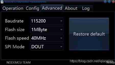
Esp8266 firmware upgrade method (esp8266-01s module)
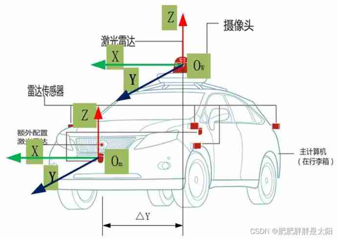
The most understandable explanation of coordinate transformation (push to + diagram)

Kotlin plug-ins kotlin Android extensions
“我被大厂裁员了”

Detailed principle of 4.3-inch TFTLCD based on warship V3
随机推荐
node:打不开/node:已拒绝访问
d的扩大@nogc
Embedded gd32 code read protection
Kali与编程:如何快速搭建OWASP网站安全实验靶场?
[data clustering] data set, visualization and precautions are involved in this column
Use of gt911 capacitive touch screen
The second revolution of reporting tools
"I was laid off by a big factory"
RT thread studio learning (VII) using multiple serial ports
Circular linked list and bidirectional linked list - practice after class
Error mcrypt in php7 version of official encryption and decryption library of enterprise wechat_ module_ Open has no method defined and is discarded by PHP. The solution is to use OpenSSL
Freshmen are worried about whether to get a low salary of more than 10000 yuan from Huawei or a high salary of more than 20000 yuan from the Internet
When SQL server2019 is installed, the next step cannot be performed. How to solve this problem?
9 Sequence container
Jackson XML is directly converted to JSON without writing entity classes manually
【图像去噪】基于高斯滤波、均值滤波、中值滤波、双边滤波四种滤波实现椒盐噪声图像去噪附matlab代码
Decoupling in D
Understanding management - four dimensions of executive power
8086/8088 instruction execution pipeline disconnection reason
Problems encountered in learning go