当前位置：网站首页>无监督图像分类《SCAN：Learning to Classify Images without》代码分析笔记（1）：simclr

无监督图像分类《SCAN：Learning to Classify Images without》代码分析笔记（1）：simclr

2022-06-11 19:21:00 【秋山丶雪绪】

前言

SCAN 分为多个步骤，本文分析第一步 simclr.py 代码。
根据论文描述，第一步为前置任务（pretext task），用于训练特征提取网络。
核心思想是对同一张图像 $P$ 变换两次得到 $P_1$ 和 $P_2$ ，通过特征提取网络输出对应特征 $T_1$ 和 $T_2$ ，最小化 $T_1$ 和 $T_2$ 特征距离（比和其他图像的特征距离近）。
代码最后阶段用 faiss 库生成 topk 用于后续步骤，因此需在 Linux 系统上运行。

simclr.py
# 输出路径
--config_env configs/env.yml
# 网络配置文件
--config_exp configs/pretext/simclr_cifar10.yml

0. 配置信息

# utils/config.py
p = create_config(args.config_env, args.config_exp)

p = 
{
    'setup': 'simclr', 
'backbone': 'resnet18', 
'model_kwargs': {
    'head': 'mlp', 'features_dim': 128}, 
'train_db_name': 'cifar-10', 
'val_db_name': 'cifar-10', 
'num_classes': 10, 
'criterion': 'simclr', 
'criterion_kwargs': {
    'temperature': 0.1}, 
'epochs': 500, 
'optimizer': 'sgd', 
'optimizer_kwargs': {
    'nesterov': False, 'weight_decay': 0.0001, 'momentum': 0.9, 'lr': 0.4}, 
'scheduler': 'cosine', 
'scheduler_kwargs': {
    'lr_decay_rate': 0.1}, 
'batch_size': 128, 
'num_workers': 8, 
'augmentation_strategy': 'simclr', 
'augmentation_kwargs': {
    'random_resized_crop': {
    'size': 32, 'scale': [0.2, 1.0]}, 
						'color_jitter_random_apply': {
    'p': 0.8}, 
						'color_jitter': {
    'brightness': 0.4, 'contrast': 0.4, 'saturation': 0.4, 'hue': 0.1}, 
						'random_grayscale': {
    'p': 0.2}, 
						'normalize': {
    'mean': [0.4914, 0.4822, 0.4465], 'std': [0.2023, 0.1994, 0.201]}}, 
'transformation_kwargs': {
    'crop_size': 32, 'normalize': {
    'mean': [0.4914, 0.4822, 0.4465], 'std': [0.2023, 0.1994, 0.201]}}, 
'pretext_dir': '/path/where/to/store/results/cifar-10\\pretext', 
'pretext_checkpoint': '/path/where/to/store/results/cifar-10\\pretext\\checkpoint.pth.tar', 
'pretext_model': '/path/where/to/store/results/cifar-10\\pretext\\model.pth.tar', 
'topk_neighbors_train_path': '/path/where/to/store/results/cifar-10\\pretext\\topk-train-neighbors.npy', 
'topk_neighbors_val_path': '/path/where/to/store/results/cifar-10\\pretext\\topk-val-neighbors.npy'}

1. Model

在这里插入图片描述
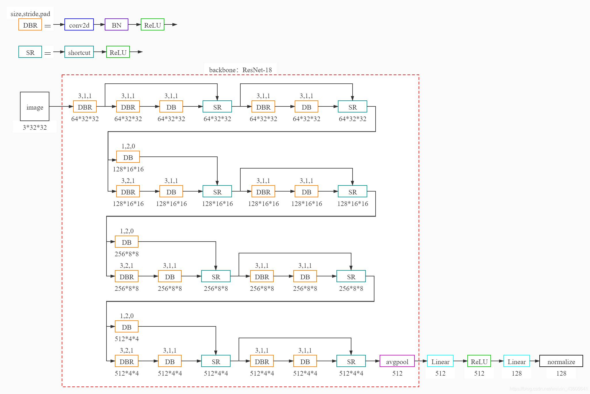
其中 normalize 为 L2_norm

model = get_model(p)  # utils/common_config.py 44

# 在 get_model(p) 中分两步构建网络
from models.resnet_cifar import resnet18
backbone = resnet18()
from models.models import ContrastiveModel
model = ContrastiveModel(backbone, **p['model_kwargs']

2. Dataset

CIFAR-10简介
数量：60000
图片尺寸：32*32
图片格式：RGB
类别数量：10
训练集：50000
测试集：10000

train_transforms = get_train_transformations(p)  # utils/common_config.py 207
val_transforms = get_val_transformations(p)  # utils/common_config.py 247

# utils/common_config.py 120
train_dataset = get_train_dataset(p, train_transforms, to_augmented_dataset=True, split='train+unlabeled') # Split is for stl-10
# utils/common_config.py 160
val_dataset = get_val_dataset(p, val_transforms)

train_dataloader = get_train_dataloader(p, train_dataset)  # utils/common_config.py 195
val_dataloader = get_val_dataloader(p, val_dataset)  # utils/common_config.py 201

训练数据中包含 image_transform 和 augmentation_transform 两个相同的随机变换方式；假设原始图像为p，p分别通过 image_transform 和 augmentation_transform 进行变换得到 p1、p2，网络输入p1、p2后得到两个特征，网络通过缩小两个特征值的差异进行学习。
图像变换方式

vars(train_dataloader)
{
    'dataset': <data.custom_dataset.AugmentedDataset object at 0x000001A883E57CC8>, 
'num_workers': 8, 
'pin_memory': True, 
'timeout': 0, 
'worker_init_fn': None, 
'_DataLoader__multiprocessing_context': None, 
'_dataset_kind': 0, 
'batch_size': 128, 
'drop_last': True, 
'sampler': <torch.utils.data.sampler.RandomSampler object at 0x000001A883CB1808>, 
'batch_sampler': <torch.utils.data.sampler.BatchSampler object at 0x000001A885466C48>, 
'collate_fn': <function collate_custom at 0x000001A8827C4168>, 
'_DataLoader__initialized': True}
----------------------------------------------------------------
vars(train_dataloader.dataset)
{
    
'dataset': <data.cifar.CIFAR10 object at 0x000001A8854503C8>, 
'image_transform': Compose(
    RandomResizedCrop(
    	size=(32, 32), 
    	scale=(0.2, 1.0), 
    	ratio=(0.75, 1.3333), 
    	interpolation=PIL.Image.BILINEAR)
   	RandomHorizontalFlip(p=0.5)
    RandomApply(
    	p=0.8
    	ColorJitter(brightness=[0.6, 1.4], contrast=[0.6, 1.4], saturation=[0.6, 1.4], hue=[-0.1, 0.1])
		)
    RandomGrayscale(p=0.2)
    ToTensor()
    Normalize(mean=[0.4914, 0.4822, 0.4465], std=[0.2023, 0.1994, 0.201])
	), 
'augmentation_transform': Compose(
    RandomResizedCrop(
    	size=(32, 32), 
    	scale=(0.2, 1.0), 
    	ratio=(0.75, 1.3333), 
    	interpolation=PIL.Image.BILINEAR)
    RandomHorizontalFlip(p=0.5)
    RandomApply(
    	p=0.8
    	ColorJitter(brightness=[0.6, 1.4], contrast=[0.6, 1.4], saturation=[0.6, 1.4], hue=[-0.1, 0.1])
		)
    RandomGrayscale(p=0.2)
    ToTensor()
    Normalize(mean=[0.4914, 0.4822, 0.4465], std=[0.2023, 0.1994, 0.201])
	)
}
----------------------------------------------------------------
vars(train_dataloader.dataset.dataset)
{
    'root': '/path/to/cifar-10/', 
'transform': None, 
'train': True, 
'classes': ['airplane', 'automobile', 'bird', 'cat', 'deer', 'dog', 'frog', 'horse', 'ship', 'truck'], 
'data': array([50000, 32, 32, 3]),
'targets':[50000],
'class_to_idx': {
    'airplane': 0, 'automobile': 1, 'bird': 2, 'cat': 3, 'deer': 4, 'dog': 5, 'frog': 6, 'horse': 7, 'ship': 8, 'truck': 9}}

vars(val_dataloader)
{
    'dataset': <data.cifar.CIFAR10 object at 0x00000207077BEA88>, 
'num_workers': 8, 
'pin_memory': True, 
'timeout': 0, 
'worker_init_fn': None, 
'_DataLoader__multiprocessing_context': None, 
'_dataset_kind': 0, 
'batch_size': 128, 
'drop_last': False, 
'sampler': <torch.utils.data.sampler.SequentialSampler object at 0x00000207077C5508>, 
'batch_sampler': <torch.utils.data.sampler.BatchSampler object at 0x00000207077C50C8>, 
'collate_fn': <function collate_custom at 0x000002070278ADC8>, 
'_DataLoader__initialized': True}
----------------------------------------------------------------
vars(val_dataloader.dataset)
{
    'root': '/path/to/cifar-10/', 
'transform': Compose(
    CenterCrop(size=(32, 32))
    ToTensor()
    Normalize(mean=[0.4914, 0.4822, 0.4465], std=[0.2023, 0.1994, 0.201])
), 
'train': False, 
'classes': ['airplane', 'automobile', 'bird', 'cat', 'deer', 'dog', 'frog', 'horse', 'ship', 'truck'], 
'data': array([10000, 32, 32, 3]),
'targets': [10000]
'class_to_idx': {
    'airplane': 0, 'automobile': 1, 'bird': 2, 'cat': 3, 'deer': 4, 'dog': 5, 'frog': 6, 'horse': 7, 'ship': 8, 'truck': 9}}

3. Memory Bank

base_dataset = get_train_dataset(p, val_transforms, split='train') # Dataset w/o augs for knn eval
base_dataloader = get_val_dataloader(p, base_dataset)
# 50000, 128, 10, 0.1
memory_bank_base = MemoryBank(len(base_dataset), 
                             p['model_kwargs']['features_dim'],
                             p['num_classes'], p['criterion_kwargs']['temperature'])
memory_bank_base.cuda()
memory_bank_val = MemoryBank(len(val_dataset),
                             p['model_kwargs']['features_dim'],
                             p['num_classes'], p['criterion_kwargs']['temperature'])
memory_bank_val.cuda()
----------------------------------------------------------------
vars(memory_bank_base)
{
    'n': 50000, 
'dim': 128, 
'features': [50000,128] tensor,
'targets': [50000] tensor,
'ptr': 0, 
'device': 'cuda:0', 
'K': 100, 
'temperature': 0.1, 
'C': 10}

4. Criterion

这部分主要负责 loss 计算，可以暂时跳过，看到 6.2 训练 部分后返回看 loss。

（1）loss 代码梳理
mask: $[b s, b s]$ 单位矩阵
contrast_features: $[b s * 2, 128]$ 两部分特征拼接
anchor: $[b s, 128]$ 第一部分特征
dot_product: $[b s, b s * 2]$ torch.matmul(anchor, contrast_features.T) / 0.1
logits: $[b s, b s * 2]$ dot_product 每行减去该行最大值，实际上就是减去左半部分主对角线的值
mask: $[b s, b s * 2]$ 变为左右两个单位矩阵
logits_mask: $[b s, b s * 2]$ 除了左半部分主对角线为0，其余全为1
mask: $[b s, b s * 2]$ 变为左半部分0矩阵，右半部分单位矩阵
exp_logits: $[b s, b s * 2]$ logits 取exp并将左半部分主对角线置0
log_prob: $[b s, b s * 2]$ logits 每行减去 exp_logits 每行的和取log
loss: log_prob 右半部分主对角线均值

（2）loss 分析
loss 的核心计算为 -log_softmax
loss 的下降可以通过缩小 $P$ 与 $P^T$ 的特征距离，以及扩大 $P$ 与除 $P^T$ 以外图像的特征距离
疑问：loss 是否会使 batch 中同类别图像特征距离扩大？或者只是在整体上 $P^T$ 的特征距离比其它的更近？

（3）点积最大值为左半部分主对角线证明
$设F_1, F_2在normalize前为\begin{bmatrix} x_1 & x_2 & \cdots & x_n \end{bmatrix}, \begin{bmatrix} y_1 & y_2 & \cdots & y_n \end{bmatrix}$
$F_1 \cdot F_2=\frac{x_1y_1+x_2y_2+\cdots+x_ny_n}{\sqrt{x_1^2+x_2^2+\cdots+x_n^2}\sqrt{y_1^2+y_2^2+\cdots+y_n^2}}$
$分母^2=\begin{matrix} x_1^2y_1^2 & x_1^2y_2^2 & \cdots & x_1^2y_n^2\\ x_2^2y_1^2 & x_2^2y_2^2 & \cdots & x_2^2y_n^2\\ \vdots & \vdots & \ddots & \vdots\\ x_n^2y_1^2 & x_n^2y_2^2 & \cdots & x_n^2y_n^2 \end{matrix}$
$分子^2=\begin{matrix} x_1^2y_1^2 & x_1y_1x_2y_2 & \cdots & x_1y_1x_ny_n\\ x_2y_2x_1y_1 & x_2^2y_2^2 & \cdots & x_2y_2x_ny_n\\ \vdots & \vdots & \ddots & \vdots\\ x_ny_nx_1y_1 & x_ny_nx_2y_2 & \cdots & x_n^2y_n^2 \end{matrix}$
$\begin{matrix} \because & 分母^2-分子^2沿主对角线看为完全平方公式 \\ \therefore & 分母^2-分子^2\ge0 \\ \therefore & 仅当 F_1=F_2 时，F_1F_2最大=1 \end{matrix}$

criterion = get_criterion(p)
criterion = criterion.cuda()

# utils/common_config.py 14
def get_criterion(p):
    if p['criterion'] == 'simclr':
        from losses.losses import SimCLRLoss
        criterion = SimCLRLoss(**p['criterion_kwargs'])

class SimCLRLoss(nn.Module):
    # Based on the implementation of SupContrast
    def __init__(self, temperature):
        super(SimCLRLoss, self).__init__()
        self.temperature = temperature
    
    def forward(self, features):
        """ input: - features: hidden feature representation of shape [b, 2, dim] output: - loss: loss computed according to SimCLR """
		b, n, dim = features.size()	# [128,2,128]
		assert(n == 2)
		mask = torch.eye(b, dtype=torch.float32).cuda()
		# torch.unbind() 删除指定维度后返回一个元组，在这里为 ([128,128],[128,128])
		# torch.cat() 按指定维度拼接，在这里为 [256,128]
		contrast_features = torch.cat(torch.unbind(features, dim=1), dim=0)	
		anchor = features[:, 0]	# anchor.size()=[128,128]
		# Dot product
		dot_product = torch.matmul(anchor, contrast_features.T) / self.temperature	# dot_product.size()=[128,256]
		# Log-sum trick for numerical stability
		logits_max, _ = torch.max(dot_product, dim=1, keepdim=True)	# logits_max.size()=[128,1]
		logits = dot_product - logits_max.detach()	# 相乘后每行减去该行的最大值

		# repeat(重复次数, 维度)
		mask = mask.repeat(1, 2)	# mask.size()=[128,256]
		# logits_mask 左半部分为1、0互换的单位矩阵右半部分为 ones 矩阵
		logits_mask = torch.scatter(torch.ones_like(mask), 1, torch.arange(b).view(-1, 1).cuda(), 0)
		mask = mask * logits_mask	# 将 mask 的左半部分变成了0矩阵，右半部分依然是单位矩阵

		# Log-softmax
		exp_logits = torch.exp(logits) * logits_mask
		log_prob = logits - torch.log(exp_logits.sum(1, keepdim=True))
        
		# Mean log-likelihood for positive
		# 实际上就是提取 log_prob 右半部分单位矩阵（左上至右下对角线）的均值
		loss = - ((mask * log_prob).sum(1) / mask.sum(1)).mean()

		return loss

5. Optimizer

optimizer = get_optimizer(p, model)

optimizer = 
SGD (
Parameter Group 0
    dampening: 0
    lr: 0.4
    momentum: 0.9
    nesterov: False
    weight_decay: 0.0001
)

6. Train

for epoch in range(start_epoch, p['epochs']):
	# Adjust lr
    lr = adjust_learning_rate(p, optimizer, epoch)
    # Train
    simclr_train(train_dataloader, model, criterion, optimizer, epoch)
    # Fill memory bank
    fill_memory_bank(base_dataloader, model, memory_bank_base)
    # Evaluate (To monitor progress - Not for validation)
    top1 = contrastive_evaluate(val_dataloader, model, memory_bank_base)

6.1 调整学习率

# Adjust lr
lr = adjust_learning_rate(p, optimizer, epoch)

# utils/common_config.py 280
def adjust_learning_rate(p, optimizer, epoch):
    lr = p['optimizer_kwargs']['lr']  # 0.4
    
    if p['scheduler'] == 'cosine':
        eta_min = lr * (p['scheduler_kwargs']['lr_decay_rate'] ** 3)  # 0.4 * (0.1 ** 3)
        lr = eta_min + (lr - eta_min) * (1 + math.cos(math.pi * epoch / p['epochs'])) / 2

    for param_group in optimizer.param_groups:
        param_group['lr'] = lr

    return lr

6.2 训练

一个 batch 的图像为 $[b s, 3, 32, 32]$
但网络的实际输入为 $[b s * 2, 3, 32, 32]$
因此网络的输出为 $[b s * 2, 128]$ ，并 resize 为 $[b s, 2, 128]$
loss 计算看 4. Criterion

simclr_train(train_dataloader, model, criterion, optimizer, epoch)

# utils/train_utils.py
def simclr_train(train_loader, model, criterion, optimizer, epoch):
    losses = AverageMeter('Loss', ':.4e')
    progress = ProgressMeter(len(train_loader),
        [losses],
        prefix="Epoch: [{}]".format(epoch))

    model.train()
    
	for i, batch in enumerate(train_loader):
		images = batch['image']
	    images_augmented = batch['image_augmented']
		b, c, h, w = images.size()	# images.size() = [128,3,32,32]
		
		input_ = torch.cat([images.unsqueeze(1), images_augmented.unsqueeze(1)], dim=1)
		# 增加一个维度然后cat, input_.size() = [128,2,3,32,32]
		input_ = input_.view(-1, c, h, w)	# input_.size() = [256,3,32,32]
		input_ = input_.cuda(non_blocking=True)
		targets = batch['target'].cuda(non_blocking=True)
		output = model(input_).view(b, 2, -1)	# output.size() = [128,2,128]
		loss = criterion(output)
        losses.update(loss.item())

        optimizer.zero_grad()
        loss.backward()
        optimizer.step()

        if i % 25 == 0:
            progress.display(i)
            
batch
{
    'image':[128,3,32,32],
'target':[128],
'meta':{
    'im_size':[2,32], 'index':[128], 'class_name':[128]},
'image_augmented':[128,3,32,32]}

6.3 Fill memory bank

得到网络对训练集（按照 val 变换）的输出特征以及标签

fill_memory_bank(base_dataloader, model, memory_bank_base)

6.4 Evaluate

验证集图像特征 $F_{\mathrm{val}}$ 与所有训练集图像特征 $F_{\mathrm{train}}$ 做点积，取出最大的100个，根据训练集标签类别索引做累加，取数值最高的索引作为 $P_{\mathrm{val}}$ 的类别，最后与 $P_{\mathrm{val}}$ 的真实标签对比计算准确度。

top1 = contrastive_evaluate(val_dataloader, model, memory_bank_base)

# utils/evaluate_utils.py
@torch.no_grad()
def contrastive_evaluate(val_loader, model, memory_bank):
    top1 = AverageMeter('[email protected]', ':6.2f')
    model.eval()

    for batch in val_loader:
        images = batch['image'].cuda(non_blocking=True)
        target = batch['target'].cuda(non_blocking=True)

        output = model(images)
        output = memory_bank.weighted_knn(output) 

        acc1 = 100*torch.mean(torch.eq(output, target).float())
        top1.update(acc1.item(), images.size(0))

    return top1.avg

class MemoryBank(object):
    def weighted_knn(self, predictions):
        # perform weighted knn
        retrieval_one_hot = torch.zeros(self.K, self.C).to(self.device)	# [100,10]
        batchSize = predictions.shape[0]
        correlation = torch.matmul(predictions, self.features.t())	# [128,128] [50000,128].T
        yd, yi = correlation.topk(self.K, dim=1, largest=True, sorted=True)	# [128,100]点积最大的前100个
        candidates = self.targets.view(1,-1).expand(batchSize, -1)	# [128,50000]
        retrieval = torch.gather(candidates, 1, yi)					# [128,100] torch.gather(索引矩阵, 索引维度, 索引)
        retrieval_one_hot.resize_(batchSize * self.K, self.C).zero_()	# [12800,10]
        retrieval_one_hot.scatter_(1, retrieval.view(-1, 1), 1)			# [12800,10] (dim, index, value)
        yd_transform = yd.clone().div_(self.temperature).exp_()
        probs = torch.sum(torch.mul(retrieval_one_hot.view(batchSize, -1 , self.C), 
                          yd_transform.view(batchSize, -1, 1)), 1)  # [128, 100, 10]*[128, 100, 1] 求和后 [128, 10]
        _, class_preds = probs.sort(1, True)
        class_pred = class_preds[:, 0]
		# 和训练集做点积，挑100个最大的统计标签，最多的为验证图像的类别
        return class_pred

7. 存储模型和 topk

# Save final model
torch.save(model.state_dict(), p['pretext_model'])

# Mine the topk nearest neighbors at the very end (Train) 
# These will be served as input to the SCAN loss.
print(colored('Fill memory bank for mining the nearest neighbors (train) ...', 'blue'))
fill_memory_bank(base_dataloader, model, memory_bank_base)
topk = 20
print('Mine the nearest neighbors (Top-%d)' %(topk)) 
indices, acc = memory_bank_base.mine_nearest_neighbors(topk)
print('Accuracy of top-%d nearest neighbors on train set is %.2f' %(topk, 100*acc))
np.save(p['topk_neighbors_train_path'], indices)   

# Mine the topk nearest neighbors at the very end (Val)
# These will be used for validation.
print(colored('Fill memory bank for mining the nearest neighbors (val) ...', 'blue'))
fill_memory_bank(val_dataloader, model, memory_bank_val)
topk = 5
print('Mine the nearest neighbors (Top-%d)' %(topk)) 
indices, acc = memory_bank_val.mine_nearest_neighbors(topk)
print('Accuracy of top-%d nearest neighbors on val set is %.2f' %(topk, 100*acc))
np.save(p['topk_neighbors_val_path'], indices)

class MemoryBank(object):
    def mine_nearest_neighbors(self, topk, calculate_accuracy=True):
        # mine the topk nearest neighbors for every sample
        import faiss
        features = self.features.cpu().numpy()
        n, dim = features.shape[0], features.shape[1]
        index = faiss.IndexFlatIP(dim)  # 点乘，归一化的向量点乘即cosine相似度（越大越好）
        index = faiss.index_cpu_to_all_gpus(index)
        index.add(features)  # 添加训练时的样本
        # indices 为相似向量的索引
        distances, indices = index.search(features, topk+1) # Sample itself is included
        
        # evaluate 
        if calculate_accuracy:
            targets = self.targets.cpu().numpy()
            neighbor_targets = np.take(targets, indices[:,1:], axis=0) # Exclude sample itself for eval
            anchor_targets = np.repeat(targets.reshape(-1,1), topk, axis=1)
            accuracy = np.mean(neighbor_targets == anchor_targets)
            return indices, accuracy
        
        else:
            return indices