当前位置:网站首页>Replace the backbone of target detection (take the fast RCNN as an example)
Replace the backbone of target detection (take the fast RCNN as an example)
2022-06-11 18:52:00 【@BangBang】
This blog uses Faster RCNN For example , Introduce how to change the target detection backbone.
For replacement target detection backbone, The main difficulty is : How to obtain the output of a feature layer in the middle of a classification network , Based on the output of the feature layer, our target detection model . Here is a brief talk about how to use pytorch The official method to build our new backbone, About building new backbone, In fact, there are many ways to do it . Let's talk about a simple method , The premise for this method is :torch>1.10
conda install pytorch==1.10.0 torchvision==0.11.0 torchaudio==0.10.0 cudatoolkit=10.2 -c pytorch
No FPN Structural replacement backbone
This blog uses Faster-RCNN The project structure of the source code is as follows :
It's going to be train_res50_fpn.py Make two copies , Named as change_backbone_with_fpn.py and change_backbone_without_fpn.py, In the copied file , The only change is create_model function . Let's talk first. change_backbone_without_fpn.py
change backbone without fpn( There is only one predictive feature layer )
No changes backbone, Corresponding train_res50_fpn.py in create_model function code :
def create_model(num_classes, load_pretrain_weights=True):
    #  Be careful , there backbone The default is FrozenBatchNorm2d, That is not to update bn Parameters
    #  The purpose is to prevent batch_size Too small makes the effect worse ( If the video memory is small , The default... Is recommended FrozenBatchNorm2d)
    #  If GPU The video memory is very large. You can set a larger batch_size It can be norm_layer Set to normal BatchNorm2d
    # trainable_layers Include ['layer4', 'layer3', 'layer2', 'layer1', 'conv1'], 5 Represents all training
    # resnet50 imagenet weights url: https://download.pytorch.org/models/resnet50-0676ba61.pth
    backbone = resnet50_fpn_backbone(pretrain_path="./backbone/resnet50.pth",
                                     norm_layer=torch.nn.BatchNorm2d,
                                     trainable_layers=3)
    #  When training your data set, don't modify the 91, The modification is the incoming num_classes Parameters
    model = FasterRCNN(backbone=backbone, num_classes=91)

    if load_pretrain_weights:
        #  Load pre training model weights
        # https://download.pytorch.org/models/fasterrcnn_resnet50_fpn_coco-258fb6c6.pth
        weights_dict = torch.load("./backbone/fasterrcnn_resnet50_fpn_coco.pth", map_location='cpu')
        missing_keys, unexpected_keys = model.load_state_dict(weights_dict, strict=False)
        if len(missing_keys) != 0 or len(unexpected_keys) != 0:
            print("missing_keys: ", missing_keys)
            print("unexpected_keys: ", unexpected_keys)

    # get number of input features for the classifier
    in_features = model.roi_heads.box_predictor.cls_score.in_features
    # replace the pre-trained head with a new one
    model.roi_heads.box_predictor = FastRCNNPredictor(in_features, num_classes)

    return model
change backbone
(1) First, in the create_model Function to import two packages
import torchvision
from torchvision.models.feature_extraction  import create_feature_extractor
Can be in pytorch Official website Check out create_feature_extractor. adopt Docs->torchvision Document found .
And retrieve create_feature_extractor, The search results are as follows :
You can view the full function description .
Example 1: backbone Replace with vgg16_bn
Here we use the official vgg16_bn, And set up pretrained=True , The pre training weight of the model will be automatically downloaded , These pre training weights are mainly for ImageNet Data sets are pre trained . Automatically load after downloading , Instantiation bakbone.
#vgg16
backbone=torchvision.models.vgg16_bn(pretrained=True)
We don't need to use the complete vgg16 Model architecture .
complete vgg16 The classification model contains a series of convolutions 、 Down sampling (max pooling) And full connection layer . In target detection , We only need the feature output of a certain layer in the middle . adopt IDE see VGG16 Source code :![[ chart ]](/img/a3/983fedbf93c884d5570e45e73a2b35.png)
In code self.features(x) Corresponding VGG From the beginning of the architecture to the dotted line , Corresponding features The last structure is max pooling layer . Take it directly self.features The output of corresponds to max pooling Results after layer output . Recommended here Down sampling 16 times The characteristic layer of , Do not use Down sampling 32 times The characteristic layer of . Because the down sampling is too large , Features are too abstract , Loss of refined features in the original drawing , It is difficult to detect some small-scale targets .
adopt VGG Architecture can know , If you just take self.features Output result , The lower sample is 32 times (224 x224 Turn into 7x7). If we want to sample 16 Times the characteristic layer , We need to get max pooling The output of the previous layer .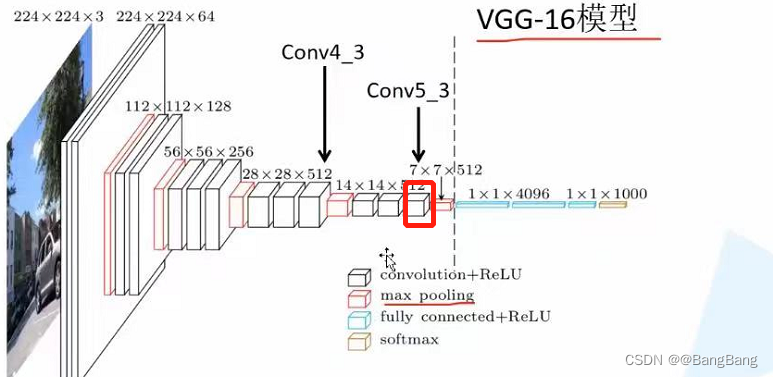
How to get the node name of the intermediate feature layer , There are two main methods : The first is to view through the source code , The second way is through print(backbone) To view the . It is easy to find the feature layer we need by looking at the source code node name , I won't introduce it here . How to set breakpoints print(backbone).
For my convenience, I will models.vgg16_bn Of pretrained Set to False, In this way, the pre training weights will not be downloaded .
Debug print out print(backbone), The results are as follows :
VGG(
  (features): Sequential(
    (0): Conv2d(3, 64, kernel_size=(3, 3), stride=(1, 1), padding=(1, 1))
    (1): BatchNorm2d(64, eps=1e-05, momentum=0.1, affine=True, track_running_stats=True)
    (2): ReLU(inplace=True)
    (3): Conv2d(64, 64, kernel_size=(3, 3), stride=(1, 1), padding=(1, 1))
    (4): BatchNorm2d(64, eps=1e-05, momentum=0.1, affine=True, track_running_stats=True)
    (5): ReLU(inplace=True)
    (6): MaxPool2d(kernel_size=2, stride=2, padding=0, dilation=1, ceil_mode=False)
    (7): Conv2d(64, 128, kernel_size=(3, 3), stride=(1, 1), padding=(1, 1))
    (8): BatchNorm2d(128, eps=1e-05, momentum=0.1, affine=True, track_running_stats=True)
    (9): ReLU(inplace=True)
    (10): Conv2d(128, 128, kernel_size=(3, 3), stride=(1, 1), padding=(1, 1))
    (11): BatchNorm2d(128, eps=1e-05, momentum=0.1, affine=True, track_running_stats=True)
    (12): ReLU(inplace=True)
    (13): MaxPool2d(kernel_size=2, stride=2, padding=0, dilation=1, ceil_mode=False)
    (14): Conv2d(128, 256, kernel_size=(3, 3), stride=(1, 1), padding=(1, 1))
    (15): BatchNorm2d(256, eps=1e-05, momentum=0.1, affine=True, track_running_stats=True)
    (16): ReLU(inplace=True)
    (17): Conv2d(256, 256, kernel_size=(3, 3), stride=(1, 1), padding=(1, 1))
    (18): BatchNorm2d(256, eps=1e-05, momentum=0.1, affine=True, track_running_stats=True)
    (19): ReLU(inplace=True)
    (20): Conv2d(256, 256, kernel_size=(3, 3), stride=(1, 1), padding=(1, 1))
    (21): BatchNorm2d(256, eps=1e-05, momentum=0.1, affine=True, track_running_stats=True)
    (22): ReLU(inplace=True)
    (23): MaxPool2d(kernel_size=2, stride=2, padding=0, dilation=1, ceil_mode=False)
    (24): Conv2d(256, 512, kernel_size=(3, 3), stride=(1, 1), padding=(1, 1))
    (25): BatchNorm2d(512, eps=1e-05, momentum=0.1, affine=True, track_running_stats=True)
    (26): ReLU(inplace=True)
    (27): Conv2d(512, 512, kernel_size=(3, 3), stride=(1, 1), padding=(1, 1))
    (28): BatchNorm2d(512, eps=1e-05, momentum=0.1, affine=True, track_running_stats=True)
    (29): ReLU(inplace=True)
    (30): Conv2d(512, 512, kernel_size=(3, 3), stride=(1, 1), padding=(1, 1))
    (31): BatchNorm2d(512, eps=1e-05, momentum=0.1, affine=True, track_running_stats=True)
    (32): ReLU(inplace=True)
    (33): MaxPool2d(kernel_size=2, stride=2, padding=0, dilation=1, ceil_mode=False)
    (34): Conv2d(512, 512, kernel_size=(3, 3), stride=(1, 1), padding=(1, 1))
    (35): BatchNorm2d(512, eps=1e-05, momentum=0.1, affine=True, track_running_stats=True)
    (36): ReLU(inplace=True)
    (37): Conv2d(512, 512, kernel_size=(3, 3), stride=(1, 1), padding=(1, 1))
    (38): BatchNorm2d(512, eps=1e-05, momentum=0.1, affine=True, track_running_stats=True)
    (39): ReLU(inplace=True)
    (40): Conv2d(512, 512, kernel_size=(3, 3), stride=(1, 1), padding=(1, 1))
    (41): BatchNorm2d(512, eps=1e-05, momentum=0.1, affine=True, track_running_stats=True)
    (42): ReLU(inplace=True)
    (43): MaxPool2d(kernel_size=2, stride=2, padding=0, dilation=1, ceil_mode=False)
  )
  (avgpool): AdaptiveAvgPool2d(output_size=(7, 7))
  (classifier): Sequential(
    (0): Linear(in_features=25088, out_features=4096, bias=True)
    (1): ReLU(inplace=True)
    (2): Dropout(p=0.5, inplace=False)
    (3): Linear(in_features=4096, out_features=4096, bias=True)
    (4): ReLU(inplace=True)
    (5): Dropout(p=0.5, inplace=False)
    (6): Linear(in_features=4096, out_features=1000, bias=True)
  )
)
From the printed structure we can see ,vgg16_bn from features,avgpool,classifier Three modules , The feature output we want is in feature The output of a sub module under a module , Correspondence is feature Module Maxpool The output of the previous layer . You can see features Under module , The index for 43 The position of corresponds to MaxPool2d Of node name . The previous node index is 42 Is the node we want features.42 Feature output .
backbone=create_feature_extractor(backbone,return_nodes={
    "features.42":"0"})
At this time, it is also necessary to backbone Set a parameter , Namely out_channels , Because in the back faster-rcnn The process of building , It needs to use backbone Output channels. About backbone.out_channels What is its output value , I offer a very simple way . First create a backbone The input of tensor, such as :batch=1,3 passageway ,224 x 224 Size picture . Then pass the data into backbone, Look at the output .
backbone=create_feature_extractor(backbone,return_nodes={
    "features.42":"0"})
out=backbone(torch.rand(1,3,224,224))
print(out["0"].shape)
Set a breakpoint , View output
You can see out It's a dictionary `` ,key yes "0" Are we in return_nodes={"features.42":"0"} Set in the key , in addition print(out["0"].shape) The output is as follows :
torch.Size([1, 512, 14, 14])
You can see the output channels=512., So set backbone.out_channels=512
backbone=create_feature_extractor(backbone,return_nodes={
    "features.42":"0"})
#out=backbone(torch.rand(1,3,224,224))
#print(out["0"].shape)
backbone.out_channels=512
It's done at this point backbone Replacement .
Example 2: Replace backbone by resnet50
In fact, the process is similar to the example 1 It's exactly the same . The complete replacement code is as follows :
# resnet50 backbone
backbone=torchvision.models.resnet50(pretrained=True)
#print(backbone)
backbone=create_feature_extractor(backbone,return_nodes={
    "layer3":"0"})
#out=backbone(torch.rand(1,3,224,224))
#print(out["0"].shape)
backbone.out_channels=1024
here return_nodes={"layer3":"0"}), Why layer3 Well ,
Click on backbone=torchvision.models.resnet50(pretrained=True) see resnet50 Source code . among forward Part of the code is as follows :
 def _forward_impl(self, x: Tensor) -> Tensor:
        # See note [TorchScript super()]
        x = self.conv1(x)
        x = self.bn1(x)
        x = self.relu(x)
        x = self.maxpool(x)

        x = self.layer1(x)
        x = self.layer2(x)
        x = self.layer3(x)
        x = self.layer4(x)

        x = self.avgpool(x)
        x = torch.flatten(x, 1)
        x = self.fc(x)

        return x

    def forward(self, x: Tensor) -> Tensor:
        return self._forward_impl(x)
there layer3 The corresponding is resnet In the network structure conv4.x Corresponding series of residual structures , Output through the network structure of this layer 14x14 Characteristic graph , It happens to be down sampling 16 times , So the corresponding key yes layer3
If you're not sure , You can debug the feature size of the printout , To verify .
 # resnet50 backbone
 backbone=torchvision.models.resnet50(pretrained=True)
 #print(backbone)
 backbone=create_feature_extractor(backbone,return_nodes={
    "layer3":"0"})
 out=backbone(torch.rand(1,3,224,224))
 print(out["0"].shape)
Output
>> torch.Size([1, 1024, 14, 14])
You can see layer3 The output of the node is 14x14, accord with 16 Double down sampling , And you can see that out_channels=1024 , So set backbone.out_channels=1024
Example 3: Replace backbone by EfficientNetB0
The method is the same as that described above , The complete code is as follows :
backbone=torchvision.models.efficientnet_b0(pretrained=False)
#print(backbone)
backbone=create_feature_extractor(backbone,return_nodes={
    "features.5":"0"})
out=backbone(torch.rand(1,3,224,224))
print(out["0"].shape)
backbone.out_channels=112
there return_nodes={"features.5":"0"}), Corresponding key by features.5
Reference blog :EfficientNet Network details 
You can see stage 6 The output characteristic is 14x14, about stage 7 Input is 14x14 , however Corresponding stride by 2 Output 7x7 Down sampling 32 times .
adopt print(backbone) Print the network structure diagram .
EfficientNet(
  (features): Sequential(
    (0): ConvNormActivation(
      (0): Conv2d(3, 32, kernel_size=(3, 3), stride=(2, 2), padding=(1, 1), bias=False)
      (1): BatchNorm2d(32, eps=1e-05, momentum=0.1, affine=True, track_running_stats=True)
      (2): SiLU(inplace=True)
    )
    (1): Sequential(
      (0): MBConv(
        (block): Sequential(
          (0): ConvNormActivation(
            (0): Conv2d(32, 32, kernel_size=(3, 3), stride=(1, 1), padding=(1, 1), groups=32, bias=False)
            (1): BatchNorm2d(32, eps=1e-05, momentum=0.1, affine=True, track_running_stats=True)
            (2): SiLU(inplace=True)
          )
          (1): SqueezeExcitation(
            (avgpool): AdaptiveAvgPool2d(output_size=1)
            (fc1): Conv2d(32, 8, kernel_size=(1, 1), stride=(1, 1))
            (fc2): Conv2d(8, 32, kernel_size=(1, 1), stride=(1, 1))
            (activation): SiLU(inplace=True)
            (scale_activation): Sigmoid()
          )
          (2): ConvNormActivation(
            (0): Conv2d(32, 16, kernel_size=(1, 1), stride=(1, 1), bias=False)
            (1): BatchNorm2d(16, eps=1e-05, momentum=0.1, affine=True, track_running_stats=True)
          )
        )
        (stochastic_depth): StochasticDepth(p=0.0, mode=row)
      )
    )
    (2): Sequential(
      (0): MBConv(
        (block): Sequential(
          (0): ConvNormActivation(
            (0): Conv2d(16, 96, kernel_size=(1, 1), stride=(1, 1), bias=False)
            (1): BatchNorm2d(96, eps=1e-05, momentum=0.1, affine=True, track_running_stats=True)
            (2): SiLU(inplace=True)
          )
          (1): ConvNormActivation(
            (0): Conv2d(96, 96, kernel_size=(3, 3), stride=(2, 2), padding=(1, 1), groups=96, bias=False)
            (1): BatchNorm2d(96, eps=1e-05, momentum=0.1, affine=True, track_running_stats=True)
            (2): SiLU(inplace=True)
          )
          (2): SqueezeExcitation(
            (avgpool): AdaptiveAvgPool2d(output_size=1)
            (fc1): Conv2d(96, 4, kernel_size=(1, 1), stride=(1, 1))
            (fc2): Conv2d(4, 96, kernel_size=(1, 1), stride=(1, 1))
            (activation): SiLU(inplace=True)
            (scale_activation): Sigmoid()
          )
          (3): ConvNormActivation(
            (0): Conv2d(96, 24, kernel_size=(1, 1), stride=(1, 1), bias=False)
            (1): BatchNorm2d(24, eps=1e-05, momentum=0.1, affine=True, track_running_stats=True)
          )
        )
        (stochastic_depth): StochasticDepth(p=0.0125, mode=row)
      )
      (1): MBConv(
        (block): Sequential(
          (0): ConvNormActivation(
            (0): Conv2d(24, 144, kernel_size=(1, 1), stride=(1, 1), bias=False)
            (1): BatchNorm2d(144, eps=1e-05, momentum=0.1, affine=True, track_running_stats=True)
            (2): SiLU(inplace=True)
          )
          (1): ConvNormActivation(
            (0): Conv2d(144, 144, kernel_size=(3, 3), stride=(1, 1), padding=(1, 1), groups=144, bias=False)
            (1): BatchNorm2d(144, eps=1e-05, momentum=0.1, affine=True, track_running_stats=True)
            (2): SiLU(inplace=True)
          )
          (2): SqueezeExcitation(
            (avgpool): AdaptiveAvgPool2d(output_size=1)
            (fc1): Conv2d(144, 6, kernel_size=(1, 1), stride=(1, 1))
            (fc2): Conv2d(6, 144, kernel_size=(1, 1), stride=(1, 1))
            (activation): SiLU(inplace=True)
            (scale_activation): Sigmoid()
          )
          (3): ConvNormActivation(
            (0): Conv2d(144, 24, kernel_size=(1, 1), stride=(1, 1), bias=False)
            (1): BatchNorm2d(24, eps=1e-05, momentum=0.1, affine=True, track_running_stats=True)
          )
        )
        (stochastic_depth): StochasticDepth(p=0.025, mode=row)
      )
    )
    (3): Sequential(
      (0): MBConv(
        (block): Sequential(
          (0): ConvNormActivation(
            (0): Conv2d(24, 144, kernel_size=(1, 1), stride=(1, 1), bias=False)
            (1): BatchNorm2d(144, eps=1e-05, momentum=0.1, affine=True, track_running_stats=True)
            (2): SiLU(inplace=True)
          )
          (1): ConvNormActivation(
            (0): Conv2d(144, 144, kernel_size=(5, 5), stride=(2, 2), padding=(2, 2), groups=144, bias=False)
            (1): BatchNorm2d(144, eps=1e-05, momentum=0.1, affine=True, track_running_stats=True)
            (2): SiLU(inplace=True)
          )
          (2): SqueezeExcitation(
            (avgpool): AdaptiveAvgPool2d(output_size=1)
            (fc1): Conv2d(144, 6, kernel_size=(1, 1), stride=(1, 1))
            (fc2): Conv2d(6, 144, kernel_size=(1, 1), stride=(1, 1))
            (activation): SiLU(inplace=True)
            (scale_activation): Sigmoid()
          )
          (3): ConvNormActivation(
            (0): Conv2d(144, 40, kernel_size=(1, 1), stride=(1, 1), bias=False)
            (1): BatchNorm2d(40, eps=1e-05, momentum=0.1, affine=True, track_running_stats=True)
          )
        )
        (stochastic_depth): StochasticDepth(p=0.037500000000000006, mode=row)
      )
      (1): MBConv(
        (block): Sequential(
          (0): ConvNormActivation(
            (0): Conv2d(40, 240, kernel_size=(1, 1), stride=(1, 1), bias=False)
            (1): BatchNorm2d(240, eps=1e-05, momentum=0.1, affine=True, track_running_stats=True)
            (2): SiLU(inplace=True)
          )
          (1): ConvNormActivation(
            (0): Conv2d(240, 240, kernel_size=(5, 5), stride=(1, 1), padding=(2, 2), groups=240, bias=False)
            (1): BatchNorm2d(240, eps=1e-05, momentum=0.1, affine=True, track_running_stats=True)
            (2): SiLU(inplace=True)
          )
          (2): SqueezeExcitation(
            (avgpool): AdaptiveAvgPool2d(output_size=1)
            (fc1): Conv2d(240, 10, kernel_size=(1, 1), stride=(1, 1))
            (fc2): Conv2d(10, 240, kernel_size=(1, 1), stride=(1, 1))
            (activation): SiLU(inplace=True)
            (scale_activation): Sigmoid()
          )
          (3): ConvNormActivation(
            (0): Conv2d(240, 40, kernel_size=(1, 1), stride=(1, 1), bias=False)
            (1): BatchNorm2d(40, eps=1e-05, momentum=0.1, affine=True, track_running_stats=True)
          )
        )
        (stochastic_depth): StochasticDepth(p=0.05, mode=row)
      )
    )
    (4): Sequential(
      (0): MBConv(
        (block): Sequential(
          (0): ConvNormActivation(
            (0): Conv2d(40, 240, kernel_size=(1, 1), stride=(1, 1), bias=False)
            (1): BatchNorm2d(240, eps=1e-05, momentum=0.1, affine=True, track_running_stats=True)
            (2): SiLU(inplace=True)
          )
          (1): ConvNormActivation(
            (0): Conv2d(240, 240, kernel_size=(3, 3), stride=(2, 2), padding=(1, 1), groups=240, bias=False)
            (1): BatchNorm2d(240, eps=1e-05, momentum=0.1, affine=True, track_running_stats=True)
            (2): SiLU(inplace=True)
          )
          (2): SqueezeExcitation(
            (avgpool): AdaptiveAvgPool2d(output_size=1)
            (fc1): Conv2d(240, 10, kernel_size=(1, 1), stride=(1, 1))
            (fc2): Conv2d(10, 240, kernel_size=(1, 1), stride=(1, 1))
            (activation): SiLU(inplace=True)
            (scale_activation): Sigmoid()
          )
          (3): ConvNormActivation(
            (0): Conv2d(240, 80, kernel_size=(1, 1), stride=(1, 1), bias=False)
            (1): BatchNorm2d(80, eps=1e-05, momentum=0.1, affine=True, track_running_stats=True)
          )
        )
        (stochastic_depth): StochasticDepth(p=0.0625, mode=row)
      )
      (1): MBConv(
        (block): Sequential(
          (0): ConvNormActivation(
            (0): Conv2d(80, 480, kernel_size=(1, 1), stride=(1, 1), bias=False)
            (1): BatchNorm2d(480, eps=1e-05, momentum=0.1, affine=True, track_running_stats=True)
            (2): SiLU(inplace=True)
          )
          (1): ConvNormActivation(
            (0): Conv2d(480, 480, kernel_size=(3, 3), stride=(1, 1), padding=(1, 1), groups=480, bias=False)
            (1): BatchNorm2d(480, eps=1e-05, momentum=0.1, affine=True, track_running_stats=True)
            (2): SiLU(inplace=True)
          )
          (2): SqueezeExcitation(
            (avgpool): AdaptiveAvgPool2d(output_size=1)
            (fc1): Conv2d(480, 20, kernel_size=(1, 1), stride=(1, 1))
            (fc2): Conv2d(20, 480, kernel_size=(1, 1), stride=(1, 1))
            (activation): SiLU(inplace=True)
            (scale_activation): Sigmoid()
          )
          (3): ConvNormActivation(
            (0): Conv2d(480, 80, kernel_size=(1, 1), stride=(1, 1), bias=False)
            (1): BatchNorm2d(80, eps=1e-05, momentum=0.1, affine=True, track_running_stats=True)
          )
        )
        (stochastic_depth): StochasticDepth(p=0.07500000000000001, mode=row)
      )
      (2): MBConv(
        (block): Sequential(
          (0): ConvNormActivation(
            (0): Conv2d(80, 480, kernel_size=(1, 1), stride=(1, 1), bias=False)
            (1): BatchNorm2d(480, eps=1e-05, momentum=0.1, affine=True, track_running_stats=True)
            (2): SiLU(inplace=True)
          )
          (1): ConvNormActivation(
            (0): Conv2d(480, 480, kernel_size=(3, 3), stride=(1, 1), padding=(1, 1), groups=480, bias=False)
            (1): BatchNorm2d(480, eps=1e-05, momentum=0.1, affine=True, track_running_stats=True)
            (2): SiLU(inplace=True)
          )
          (2): SqueezeExcitation(
            (avgpool): AdaptiveAvgPool2d(output_size=1)
            (fc1): Conv2d(480, 20, kernel_size=(1, 1), stride=(1, 1))
            (fc2): Conv2d(20, 480, kernel_size=(1, 1), stride=(1, 1))
            (activation): SiLU(inplace=True)
            (scale_activation): Sigmoid()
          )
          (3): ConvNormActivation(
            (0): Conv2d(480, 80, kernel_size=(1, 1), stride=(1, 1), bias=False)
            (1): BatchNorm2d(80, eps=1e-05, momentum=0.1, affine=True, track_running_stats=True)
          )
        )
        (stochastic_depth): StochasticDepth(p=0.08750000000000001, mode=row)
      )
    )
    (5): Sequential(
      (0): MBConv(
        (block): Sequential(
          (0): ConvNormActivation(
            (0): Conv2d(80, 480, kernel_size=(1, 1), stride=(1, 1), bias=False)
            (1): BatchNorm2d(480, eps=1e-05, momentum=0.1, affine=True, track_running_stats=True)
            (2): SiLU(inplace=True)
          )
          (1): ConvNormActivation(
            (0): Conv2d(480, 480, kernel_size=(5, 5), stride=(1, 1), padding=(2, 2), groups=480, bias=False)
            (1): BatchNorm2d(480, eps=1e-05, momentum=0.1, affine=True, track_running_stats=True)
            (2): SiLU(inplace=True)
          )
          (2): SqueezeExcitation(
            (avgpool): AdaptiveAvgPool2d(output_size=1)
            (fc1): Conv2d(480, 20, kernel_size=(1, 1), stride=(1, 1))
            (fc2): Conv2d(20, 480, kernel_size=(1, 1), stride=(1, 1))
            (activation): SiLU(inplace=True)
            (scale_activation): Sigmoid()
          )
          (3): ConvNormActivation(
            (0): Conv2d(480, 112, kernel_size=(1, 1), stride=(1, 1), bias=False)
            (1): BatchNorm2d(112, eps=1e-05, momentum=0.1, affine=True, track_running_stats=True)
          )
        )
        (stochastic_depth): StochasticDepth(p=0.1, mode=row)
      )
      (1): MBConv(
        (block): Sequential(
          (0): ConvNormActivation(
            (0): Conv2d(112, 672, kernel_size=(1, 1), stride=(1, 1), bias=False)
            (1): BatchNorm2d(672, eps=1e-05, momentum=0.1, affine=True, track_running_stats=True)
            (2): SiLU(inplace=True)
          )
          (1): ConvNormActivation(
            (0): Conv2d(672, 672, kernel_size=(5, 5), stride=(1, 1), padding=(2, 2), groups=672, bias=False)
            (1): BatchNorm2d(672, eps=1e-05, momentum=0.1, affine=True, track_running_stats=True)
            (2): SiLU(inplace=True)
          )
          (2): SqueezeExcitation(
            (avgpool): AdaptiveAvgPool2d(output_size=1)
            (fc1): Conv2d(672, 28, kernel_size=(1, 1), stride=(1, 1))
            (fc2): Conv2d(28, 672, kernel_size=(1, 1), stride=(1, 1))
            (activation): SiLU(inplace=True)
            (scale_activation): Sigmoid()
          )
          (3): ConvNormActivation(
            (0): Conv2d(672, 112, kernel_size=(1, 1), stride=(1, 1), bias=False)
            (1): BatchNorm2d(112, eps=1e-05, momentum=0.1, affine=True, track_running_stats=True)
          )
        )
        (stochastic_depth): StochasticDepth(p=0.1125, mode=row)
      )
      (2): MBConv(
        (block): Sequential(
          (0): ConvNormActivation(
            (0): Conv2d(112, 672, kernel_size=(1, 1), stride=(1, 1), bias=False)
            (1): BatchNorm2d(672, eps=1e-05, momentum=0.1, affine=True, track_running_stats=True)
            (2): SiLU(inplace=True)
          )
          (1): ConvNormActivation(
            (0): Conv2d(672, 672, kernel_size=(5, 5), stride=(1, 1), padding=(2, 2), groups=672, bias=False)
            (1): BatchNorm2d(672, eps=1e-05, momentum=0.1, affine=True, track_running_stats=True)
            (2): SiLU(inplace=True)
          )
          (2): SqueezeExcitation(
            (avgpool): AdaptiveAvgPool2d(output_size=1)
            (fc1): Conv2d(672, 28, kernel_size=(1, 1), stride=(1, 1))
            (fc2): Conv2d(28, 672, kernel_size=(1, 1), stride=(1, 1))
            (activation): SiLU(inplace=True)
            (scale_activation): Sigmoid()
          )
          (3): ConvNormActivation(
            (0): Conv2d(672, 112, kernel_size=(1, 1), stride=(1, 1), bias=False)
            (1): BatchNorm2d(112, eps=1e-05, momentum=0.1, affine=True, track_running_stats=True)
          )
        )
        (stochastic_depth): StochasticDepth(p=0.125, mode=row)
      )
    )
    (6): Sequential(
      (0): MBConv(
        (block): Sequential(
          (0): ConvNormActivation(
            (0): Conv2d(112, 672, kernel_size=(1, 1), stride=(1, 1), bias=False)
            (1): BatchNorm2d(672, eps=1e-05, momentum=0.1, affine=True, track_running_stats=True)
            (2): SiLU(inplace=True)
          )
          (1): ConvNormActivation(
            (0): Conv2d(672, 672, kernel_size=(5, 5), stride=(2, 2), padding=(2, 2), groups=672, bias=False)
            (1): BatchNorm2d(672, eps=1e-05, momentum=0.1, affine=True, track_running_stats=True)
            (2): SiLU(inplace=True)
          )
          (2): SqueezeExcitation(
            (avgpool): AdaptiveAvgPool2d(output_size=1)
            (fc1): Conv2d(672, 28, kernel_size=(1, 1), stride=(1, 1))
            (fc2): Conv2d(28, 672, kernel_size=(1, 1), stride=(1, 1))
            (activation): SiLU(inplace=True)
            (scale_activation): Sigmoid()
          )
          (3): ConvNormActivation(
            (0): Conv2d(672, 192, kernel_size=(1, 1), stride=(1, 1), bias=False)
            (1): BatchNorm2d(192, eps=1e-05, momentum=0.1, affine=True, track_running_stats=True)
          )
        )
        (stochastic_depth): StochasticDepth(p=0.1375, mode=row)
      )
      (1): MBConv(
        (block): Sequential(
          (0): ConvNormActivation(
            (0): Conv2d(192, 1152, kernel_size=(1, 1), stride=(1, 1), bias=False)
            (1): BatchNorm2d(1152, eps=1e-05, momentum=0.1, affine=True, track_running_stats=True)
            (2): SiLU(inplace=True)
          )
          (1): ConvNormActivation(
            (0): Conv2d(1152, 1152, kernel_size=(5, 5), stride=(1, 1), padding=(2, 2), groups=1152, bias=False)
            (1): BatchNorm2d(1152, eps=1e-05, momentum=0.1, affine=True, track_running_stats=True)
            (2): SiLU(inplace=True)
          )
          (2): SqueezeExcitation(
            (avgpool): AdaptiveAvgPool2d(output_size=1)
            (fc1): Conv2d(1152, 48, kernel_size=(1, 1), stride=(1, 1))
            (fc2): Conv2d(48, 1152, kernel_size=(1, 1), stride=(1, 1))
            (activation): SiLU(inplace=True)
            (scale_activation): Sigmoid()
          )
          (3): ConvNormActivation(
            (0): Conv2d(1152, 192, kernel_size=(1, 1), stride=(1, 1), bias=False)
            (1): BatchNorm2d(192, eps=1e-05, momentum=0.1, affine=True, track_running_stats=True)
          )
        )
        (stochastic_depth): StochasticDepth(p=0.15000000000000002, mode=row)
      )
      (2): MBConv(
        (block): Sequential(
          (0): ConvNormActivation(
            (0): Conv2d(192, 1152, kernel_size=(1, 1), stride=(1, 1), bias=False)
            (1): BatchNorm2d(1152, eps=1e-05, momentum=0.1, affine=True, track_running_stats=True)
            (2): SiLU(inplace=True)
          )
          (1): ConvNormActivation(
            (0): Conv2d(1152, 1152, kernel_size=(5, 5), stride=(1, 1), padding=(2, 2), groups=1152, bias=False)
            (1): BatchNorm2d(1152, eps=1e-05, momentum=0.1, affine=True, track_running_stats=True)
            (2): SiLU(inplace=True)
          )
          (2): SqueezeExcitation(
            (avgpool): AdaptiveAvgPool2d(output_size=1)
            (fc1): Conv2d(1152, 48, kernel_size=(1, 1), stride=(1, 1))
            (fc2): Conv2d(48, 1152, kernel_size=(1, 1), stride=(1, 1))
            (activation): SiLU(inplace=True)
            (scale_activation): Sigmoid()
          )
          (3): ConvNormActivation(
            (0): Conv2d(1152, 192, kernel_size=(1, 1), stride=(1, 1), bias=False)
            (1): BatchNorm2d(192, eps=1e-05, momentum=0.1, affine=True, track_running_stats=True)
          )
        )
        (stochastic_depth): StochasticDepth(p=0.1625, mode=row)
      )
      (3): MBConv(
        (block): Sequential(
          (0): ConvNormActivation(
            (0): Conv2d(192, 1152, kernel_size=(1, 1), stride=(1, 1), bias=False)
            (1): BatchNorm2d(1152, eps=1e-05, momentum=0.1, affine=True, track_running_stats=True)
            (2): SiLU(inplace=True)
          )
          (1): ConvNormActivation(
            (0): Conv2d(1152, 1152, kernel_size=(5, 5), stride=(1, 1), padding=(2, 2), groups=1152, bias=False)
            (1): BatchNorm2d(1152, eps=1e-05, momentum=0.1, affine=True, track_running_stats=True)
            (2): SiLU(inplace=True)
          )
          (2): SqueezeExcitation(
            (avgpool): AdaptiveAvgPool2d(output_size=1)
            (fc1): Conv2d(1152, 48, kernel_size=(1, 1), stride=(1, 1))
            (fc2): Conv2d(48, 1152, kernel_size=(1, 1), stride=(1, 1))
            (activation): SiLU(inplace=True)
            (scale_activation): Sigmoid()
          )
          (3): ConvNormActivation(
            (0): Conv2d(1152, 192, kernel_size=(1, 1), stride=(1, 1), bias=False)
            (1): BatchNorm2d(192, eps=1e-05, momentum=0.1, affine=True, track_running_stats=True)
          )
        )
        (stochastic_depth): StochasticDepth(p=0.17500000000000002, mode=row)
      )
    )
    (7): Sequential(
      (0): MBConv(
        (block): Sequential(
          (0): ConvNormActivation(
            (0): Conv2d(192, 1152, kernel_size=(1, 1), stride=(1, 1), bias=False)
            (1): BatchNorm2d(1152, eps=1e-05, momentum=0.1, affine=True, track_running_stats=True)
            (2): SiLU(inplace=True)
          )
          (1): ConvNormActivation(
            (0): Conv2d(1152, 1152, kernel_size=(3, 3), stride=(1, 1), padding=(1, 1), groups=1152, bias=False)
            (1): BatchNorm2d(1152, eps=1e-05, momentum=0.1, affine=True, track_running_stats=True)
            (2): SiLU(inplace=True)
          )
          (2): SqueezeExcitation(
            (avgpool): AdaptiveAvgPool2d(output_size=1)
            (fc1): Conv2d(1152, 48, kernel_size=(1, 1), stride=(1, 1))
            (fc2): Conv2d(48, 1152, kernel_size=(1, 1), stride=(1, 1))
            (activation): SiLU(inplace=True)
            (scale_activation): Sigmoid()
          )
          (3): ConvNormActivation(
            (0): Conv2d(1152, 320, kernel_size=(1, 1), stride=(1, 1), bias=False)
            (1): BatchNorm2d(320, eps=1e-05, momentum=0.1, affine=True, track_running_stats=True)
          )
        )
        (stochastic_depth): StochasticDepth(p=0.1875, mode=row)
      )
    )
    (8): ConvNormActivation(
      (0): Conv2d(320, 1280, kernel_size=(1, 1), stride=(1, 1), bias=False)
      (1): BatchNorm2d(1280, eps=1e-05, momentum=0.1, affine=True, track_running_stats=True)
      (2): SiLU(inplace=True)
    )
  )
  (avgpool): AdaptiveAvgPool2d(output_size=1)
  (classifier): Sequential(
    (0): Dropout(p=0.2, inplace=True)
    (1): Linear(in_features=1280, out_features=1000, bias=True)
  )
)
Network structure stage 6, For and features Under module , The index for 5 Sub module of , So the corresponding node is "features.5"
structure Faster RCNN Code explanation
structure backbone
Create good backbone after , Next, let's talk about how to build Faster RCNN Model , What is introduced here is without FPN Structural , That is to say, there is only one prediction feature layer .
Instantiation AnchorGenerator and roi_pooler
Instantiation AnchorGenerator
 anchor_generator = AnchorsGenerator(sizes=((32, 64, 128, 256, 512),),
                                        aspect_ratios=((0.5, 1.0, 2.0),))
Pass in two parameters , One is sizes, One is aspect_ratios. size and aspect_ratios They are all Yuanzu types , And they are all one element , Because we are building without FPN Structure , There is only one predictive feature layer , Corresponding sizes and aspect_ratios Yuanzu had only one element
If we don't define here AnchorGenerator, stay Faster RCNN Internally, it will be built automatically for FPN Structural AnchorGenerator as well as roi_pooler, So we need to build in advance AnchorGenerator and roi_pooler
 anchor_generator = AnchorsGenerator(sizes=((32, 64, 128, 256, 512),),
                                        aspect_ratios=((0.5, 1.0, 2.0),))

roi_pooler = torchvision.ops.MultiScaleRoIAlign(featmap_names=['0'],  #  On which feature layers RoIAlign pooling
                                                  output_size=[7, 7],  # RoIAlign pooling Output characteristic matrix size
                                                  sampling_ratio=2)  #  Sampling rate
Used here MutiScaleRoIAlign , This is relative Faster RCNN What the thesis is about RoiPooler It will be more accurate . Because there's only one key by 0 Prediction characteristic layer of , So in MultiScaleRoIAlign In the middle of featmap_names=['0']
model building
Build the model :
 model = FasterRCNN(backbone=backbone,
                       num_classes=num_classes,
                       rpn_anchor_generator=anchor_generator,
                       box_roi_pool=roi_pooler)
The complete code is as follows :
def create_model(num_classes, load_pretrain_weights=True):
    import torchvision
    from torchvision.models.feature_extraction import create_feature_extractor

    # vgg16
    backbone=torchvision.models.vgg16_bn(pretrained=False)
    print(backbone)

    backbone=create_feature_extractor(backbone,return_nodes={
    "features.42":"0"})
    #out=backbone(torch.rand(1,3,224,224))
    #print(out["0"].shape)
    backbone.out_channels=512

    # resnet50 backbone
    # backbone=torchvision.models.resnet50(pretrained=False)
    # #print(backbone)
    # backbone=create_feature_extractor(backbone,return_nodes={"layer3":"0"})
    # out=backbone(torch.rand(1,3,224,224))
    # print(out["0"].shape)
    # backbone.out_channels=1024

    # efficientnet_b0 backbone
    # backbone=torchvision.models.efficientnet_b0(pretrained=False)
    # print(backbone)
    # backbone=create_feature_extractor(backbone,return_nodes={"features.5":"0"})
    # out=backbone(torch.rand(1,3,224,224))
    # print(out["0"].shape)
    # backbone.out_channels=112

    anchor_generator = AnchorsGenerator(sizes=((32, 64, 128, 256, 512),),
                                        aspect_ratios=((0.5, 1.0, 2.0),))

    roi_pooler = torchvision.ops.MultiScaleRoIAlign(featmap_names=['0'],  #  On which feature layers RoIAlign pooling
                                                    output_size=[7, 7],  # RoIAlign pooling Output characteristic matrix size
                                                    sampling_ratio=2)  #  Sampling rate

    model = FasterRCNN(backbone=backbone,
                       num_classes=num_classes,
                       rpn_anchor_generator=anchor_generator,
                       box_roi_pool=roi_pooler)

    return model
belt FPN Structural replacement backbone
The corresponding code is in change_backbone_with_fpn.py In file , Similarly, let's look at create_model This part of the code .
First, in the create_model Function to import two packages
import torchvision
from torchvision.models.feature_extraction  import create_feature_extractor
What we use pytorch Version must be 1.10 Or more ,torchvision Also follow and pytorch Corresponding version
Replace backbone
With mobienet_v3_large backbone For example
# --- mobilenet_v3_large fpn backbone --- #
backbone = torchvision.models.mobilenet_v3_large(pretrained=True)
Set up pretrained=True, During the process of creating the model, it will be automatically downloaded in ImageNet Pre trained weights .
Construction zone fpn Structural backbone, Reference resources object detection FPN Use of structure ,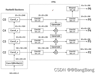
The main difficulty is to know which feature layers we want to acquire , And these feature layers correspond to the output of which module .
return_layers = {
    "features.6": "0",   # stride 8
                  "features.12": "1",  # stride 16
                  "features.16": "2"}  # stride 32
Created a return_layers Dictionaries , Each key value pair in the dictionary corresponds to a certain feature layer , And without FPN Of backbone similar , Just take FPN Structural backbone It is necessary to extract multiple special positive layers .
- key The corresponding feature layer is extracted , Node location in the network
- value, Default settings from "0" Began to increase
![[MobileNetV3-Large chart ]](/img/7e/47300ffae6ea8ba309cc36a21b2396.png)
This picture is the original paper for MobileNetV3-Large A structure of a network , Suppose I want to get the blue box in the figure 3 Outputs corresponding to modules , As you can see, for the first module, we sampled 8 times , The second module samples 16 times , The third module samples 32 times . Of course, you can also select appropriate modules to extract features according to your own ideas .
How to find the extracted 3 The name of each module ? There are two main ways :
- The first is to view through the source code
- The second way is through
print(backbone)To view the .
adopt IDE See build MobileNetV3-Large Source code , We can see what the authorities have achieved features
self.features = nn.Sequential(*layers)
What it stores is the corresponding index in the above figure 0-16 Of 17 A module , In the source code, we can know that each layer will add a module , So the corresponding index is where the module is located . The modules extracted from the figure , The corresponding is 6,12,16 , If you are not clear, you can also print backbone To view the .
Set it up return_layers after , We also need to specify the feature layers we extract , They correspond to channels, From the table in the figure above, you can see that this layer corresponds to channels, Namely [40,112,960], If you don't know chanel Words , I create one randomly tensor, Input backbone, Then, the feature layer names and shape.
backbone = torchvision.models.mobilenet_v3_large(pretrained=False)
print(backbone)
return_layers = {
    "features.6": "0",   # stride 8
                 "features.12": "1",  # stride 16
                 "features.16": "2"}  # stride 32
#  Provide to fpn Each feature layer channel
# in_channels_list = [40, 112, 960]
new_backbone = create_feature_extractor(backbone, return_layers)
img = torch.randn(1, 3, 224, 224)
outputs = new_backbone(img)
[print(f"{
      k} shape: {
      v.shape}") for k, v in outputs.items()]
Printed information :
0 shape: torch.Size([1, 40, 28, 28])
1 shape: torch.Size([1, 112, 14, 14])
2 shape: torch.Size([1, 960, 7, 7])
there key 0,1,2 Are we in retrun_layers As defined in value. The channels can be seen as 40,112,960, Combine the output height and width values of each feature layer , It can help us analyze whether the down sampling ratio of the feature layer we extracted is correct .
Next , By instantiating backboneWithFPN To build the belt fpn Of backbone.
backbone_with_fpn = BackboneWithFPN(new_backbone,
                                        return_layers=return_layers,
                                        in_channels_list=in_channels_list,
                                        out_channels=256,
                                        extra_blocks=LastLevelMaxPool(),
                                        re_getter=False)
There will be re_getter Set to False You won't refactor the model ,Direct use ofcreate_feature_extractor(backbone, return_layers)Instantiated new_backbone, Because of the use of BackboneWithFPN It can't get something layers Output of sub module under , So usecreate_feature_extractor(backbone, return_layers)To reconstruct backbone It will be more convenient and flexible .Pass in return_layers,in_channel_list
out_channels by 256, We are building fpn Of each feature layer channel adopt 1x1 The convolution of is adjusted to 256

extra_blocks=LastLevelMaxPool, Its function is what we draw in the picture , In the top feature layer , Through a Maxpool Take an upper sample . Get a smaller feature layer . A smaller feature layer helps us detect larger targets . And there is one more thing to note here Maxpool The obtained feature layer , It is only for our RPN part , be not in Fast-RCNN Use in .
And then use it FeaturePyramidNetwork To build fpn structure
 self.fpn = FeaturePyramidNetwork(
            in_channels_list=in_channels_list,
            out_channels=out_channels,
            extra_blocks=extra_blocks,
        )
From the forward propagation, we can see , It uses input data , Pass... In turn boy That is, after the refactoring backbone, and fpn Then we get our output .
class BackboneWithFPN(nn.Module):
    def __init__(self,
                 backbone: nn.Module,
                 return_layers=None,
                 in_channels_list=None,
                 out_channels=256,
                 extra_blocks=None,
                 re_getter=True):
        super().__init__()

        if extra_blocks is None:
            extra_blocks = LastLevelMaxPool()

        if re_getter is True:
            assert return_layers is not None
            self.body = IntermediateLayerGetter(backbone, return_layers=return_layers)
        else:
            self.body = backbone

        self.fpn = FeaturePyramidNetwork(
            in_channels_list=in_channels_list,
            out_channels=out_channels,
            extra_blocks=extra_blocks,
        )

        self.out_channels = out_channels

    def forward(self, x):
        x = self.body(x)
        x = self.fpn(x)
        return x
To complete the BackboneWithFPN Of backbone The construction of
AnchorGenerator and aspect_ratios
 anchor_sizes = ((64,), (128,), (256,), (512,))
 aspect_ratios = ((0.5, 1.0, 2.0),) * len(anchor_sizes)
 anchor_generator = AnchorsGenerator(sizes=anchor_sizes,
                                     aspect_ratios=aspect_ratios)
                                       roi_pooler = torchvision.ops.MultiScaleRoIAlign(featmap_names=['0', '1', '2'],  #  On which feature layers RoIAlign pooling
                                                    output_size=[7, 7],  # RoIAlign pooling Output characteristic matrix size
                                                    sampling_ratio=2)  #  Sampling rate
- Here for each feature layer , Only one has been set anchor scale , For example, for the feature layer with the largest scale , Used to detect small targets , Set the scale to 64, A medium-sized feature layer will anchor Set to 128, The characteristic layer of the relatively high level anchor The size is set to 256, Finally through maxpool The resulting feature layer is 512
- For each feature layer , Set up (0.5,1.0,2.0) These three ratios
- MultiScaleRoIAlign Is in Fast-RCNN Used in ,feature_names Defines that RPN Structure generated perposal To which feature layers ., Why... Here maxpool Layer is not used , Because this layer is only used for RPN part , be not in Fast-RCNN Some use .
- output_size Explain how big we will sample
- sampling_rate Define our sampling rate
Defined with FPN Of backbone, as well as anchor_generator, roi_pooler, So we can create FasterRCNN 了
  model = FasterRCNN(backbone=backbone_with_fpn,
                       num_classes=num_classes,
                       rpn_anchor_generator=anchor_generator,
                       box_roi_pool=roi_pooler)
Complete with FPN Structural FasterRCNN The code is as follows :
def create_model(num_classes):
    import torchvision
    from torchvision.models.feature_extraction import create_feature_extractor

    # --- mobilenet_v3_large fpn backbone --- #
    backbone = torchvision.models.mobilenet_v3_large(pretrained=False)
    print(backbone)
    return_layers = {
    "features.6": "0",   # stride 8
                     "features.12": "1",  # stride 16
                     "features.16": "2"}  # stride 32
    #  Provide to fpn Each feature layer channel
    # in_channels_list = [40, 112, 960]
    new_backbone = create_feature_extractor(backbone, return_layers)
    img = torch.randn(1, 3, 224, 224)
    outputs = new_backbone(img)
    [print(f"{
      k} shape: {
      v.shape}") for k, v in outputs.items()]

    # --- efficientnet_b0 fpn backbone --- #
    # backbone = torchvision.models.efficientnet_b0(pretrained=True)
    # # print(backbone)
    # return_layers = {"features.3": "0", # stride 8
    # "features.4": "1", # stride 16
    # "features.8": "2"} # stride 32
    # #  Provide to fpn Each feature layer channel
    # in_channels_list = [40, 80, 1280]
    # new_backbone = create_feature_extractor(backbone, return_layers)
    # # img = torch.randn(1, 3, 224, 224)
    # # outputs = new_backbone(img)
    # # [print(f"{k} shape: {v.shape}") for k, v in outputs.items()]

    backbone_with_fpn = BackboneWithFPN(new_backbone,
                                        return_layers=return_layers,
                                        in_channels_list=in_channels_list,
                                        out_channels=256,
                                        extra_blocks=LastLevelMaxPool(),
                                        re_getter=False)

    anchor_sizes = ((64,), (128,), (256,), (512,))
    aspect_ratios = ((0.5, 1.0, 2.0),) * len(anchor_sizes)
    anchor_generator = AnchorsGenerator(sizes=anchor_sizes,
                                        aspect_ratios=aspect_ratios)

    roi_pooler = torchvision.ops.MultiScaleRoIAlign(featmap_names=['0', '1', '2'],  #  On which feature layers RoIAlign pooling
                                                    output_size=[7, 7],  # RoIAlign pooling Output characteristic matrix size
                                                    sampling_ratio=2)  #  Sampling rate

    model = FasterRCNN(backbone=backbone_with_fpn,
                       num_classes=num_classes,
                       rpn_anchor_generator=anchor_generator,
                       box_roi_pool=roi_pooler)

    return model
Be careful : It's over backbone after , Use it to train your data set directly , The general effect will be poor , Because we only load backbone Partial pre training weights , Yes FPN,RPN as well as Fast RCNN Part of the weight we have not learned , The effect of directly training your own data set is generally poor .
Suggest : First take the model you have built and put it in coco Pre-training on the data set , After pre training, take your own data for migration learning , Can achieve better results .
Source download
边栏推荐
- 制造出静态坦克
- 2023年西安交通大学管理学院MPAcc提前批面试网报通知
- *Use of jetpack notes room
- 手把手教你学会FIRST集和FOLLOW集!!!!吐血收藏!!保姆级讲解!!!
- Labelme for image data annotation
- 对‘g2o::VertexSE3::VertexSE3()’未定义的引用
- Force buckle 34 finds the first and last positions of elements in a sorted array
- SAP UI5 里 XML 视图根节点运行时实例化的分析
- 全国院校MBA、EMBA、MPA、MEM、提前面试(预面试)时间批次已出(持续更新中)-文都管联院
- Overall process of software development
猜你喜欢

一款自适应的聊天网站-匿名在线聊天室PHP源码

BigDecimal基本使用与闭坑介绍

Map and set

北京邮电大学2023级工商管理硕士MBA(非全日制)已开启

全志科技T3开发板(4核ARM Cortex-A7)——视频开发案例

cf:D. Black and White Stripe【连续k个中最少的个数 + 滑动窗口】
Cf:d. black and white stripe

WWDC22 开发者需要关注的重点内容
全国院校MBA、EMBA、MPA、MEM、提前面试(预面试)时间批次已出(持续更新中)-文都管联院

SQL injection vulnerability learning 1: phpstudy integrated environment building DVWA shooting range
随机推荐
力扣刷题——根据二叉树创建字符串
Construct enemy tanks
牛客刷题——把字符串转换成整数
如何在 SAP BTP 上 手动执行 workflow
Monitoring loss functions using visdom
An adaptive chat site - anonymous online chat room PHP source code
TI AM64x——最新16nm处理平台,专为工业网关、工业机器人而生
Let our tanks move happily
Force deduction 23 questions, merging K ascending linked lists
Ubuntu installs PSQL and runs related commands
SQL injection vulnerability learning 1: phpstudy integrated environment building DVWA shooting range
The 2023 MBA (Part-time) of Beijing University of Posts and telecommunications has been launched
Introduction to basic use and pit closure of BigDecimal
力扣刷题——二叉树的最近公共祖先
Prevent enemy tanks from overlapping
Niu Ke brushes the question - no two
Niu Ke swipes the question -- converting a string to an integer
cf:A. Print a Pedestal (Codeforces logo?) [simple traversal simulation]
leetcode:926. Flip the string to monotonically increasing [prefix and + analog analysis]
Quanzhi Technology T3 Development Board (4 Core ARM Cortex - A7) - mqtt Communication Protocol case