Carry forward the past and forge ahead into the future, multiple residuals | densenet (I)

Densely connected convolutional networks

Thesis title ：Densely Connected Convolutional Networks

paper It was published by Cornell University in CVPR 2017 Work on

Address of thesis ： link

Abstract

Recent work shows that , If the convolution network contains a short connection between the layer close to the input and the layer close to the output , Then they can be deeper 、 Train more accurately and effectively . This paper accepts this observation and introduces dense convolutional networks （DenseNet）, It connects each layer to every other layer in a feedforward way . have $L$ The traditional convolution network of layer has $L$ A connection —— There is a connection between each layer and its subsequent layers —— The network of this article includes $\frac{L(L+1)}{2}$ A direct connection . For each layer , All front level feature maps are used as input , Its own characteristic graph is used as input for all subsequent layers .DenseNets There are several advantages ： It alleviates the gradient vanishing problem , Enhanced feature dissemination , Encourage feature reuse , And greatly reduce the number of parameters . The author worked on four target recognition benchmark tasks （CIF AR-10、CIF AR-100、SVHN and ImageNet） To evaluate the proposed architecture .DenseNets In most respects, it is better than the most advanced technology , At the same time, less computation is required , High performance . The code and pre training model are published in ：github link

1. Introduction

Convolutional neural networks (CNN) It has become the main machine learning method for visual target recognition . Although they were originally 20 Introduced many years ago , But the improvement of computer hardware and network structure has not been able to train real depth until recently CNN. The original LeNet5 Yes 5 layer ,VGG Yes 19 layer , Until last year , Expressway Network (Highway Networks) And the residual network (ResNets) Just across 100 Layer obstacles .

With CNN It's getting deeper and deeper , A new research problem has emerged ： When information about inputs or gradients passes through many layers , It may reach the end of the network （ Or start ） Disappear and “wash out”. A lot of recent work has been done to solve this or related problems . ResNets and Highway Networks Bypass the signal from one layer to the next through an identity connection .Stochastic depth Randomly discard layers during training to shorten ResNet, To provide better information and gradient flow . FractalNets Multiple parallel layer sequences are combined repeatedly with different numbers of convolution blocks to obtain larger nominal depth , At the same time, keep many short paths in the network . Although these methods are different in network topology and training process , But they all have a key feature ： They create short paths from shallow to deep .

This paper presents an architecture , Put this insight Refine it into a simple connection pattern ： In order to ensure the maximum information flow between layers in the network , Put all layers （ Matching feature map size ） Directly connected to each other . In order to maintain the feedforward property , Each layer gets additional input from all previous layers , And pass its own characteristic graph to all subsequent layers . chart 1 This layout is illustrated . It is important to , And ResNets comparison , Before transferring the feature to the layer, start from Not by summation To combine features . But through Connect （concat） They combine features . therefore , The first ${\ell }^{th}$ Layer has a $\ell$ Inputs , It consists of characteristic graphs of all previous convolution blocks . Its own feature map is passed to all $L-\ell$ Subsequent layers . This is in $L$ Layer network $\frac{L(L+1)}{2}$ A connection , Instead of just introducing... As in traditional architectures $L$ A connection . Because of its dense connection mode , The method in this paper is called dense convolution network （DenseNet）.

chart 1： The growth rate is $k=4$ Of 5 Layer dense block . Each layer takes all previous feature maps as input .

One possible counterintuitive effect of this dense connection pattern is , Compared with the traditional convolution network , It requires fewer parameters , Because there is no need to relearn redundant characteristic graphs . The traditional feedforward architecture can be regarded as a stateful algorithm , This state is passed from layer to layer . Each layer reads the state from its previous layer and writes it to subsequent layers . It changed the State , But it also conveys information that needs to be preserved .ResNets Through the additive identity transformation, the information preservation becomes clear . ResNets The latest variant of shows , Many layers contribute little , In fact, it can be discarded randomly during training . This makes ResNets The state of is similar to （ In the ） Cyclic neural network , but ResNets The parameter quantity of is much larger , Because each layer has its own weight .DenseNet framework A clear distinction is made between information added to the network and information retained . DenseNet The layer is very narrow （ for example , Each layer 12 A filter ）, Add only a small part of the feature map to the “collective knowledge” in , And keep the other characteristic figures unchanged , The final classifier makes a decision based on all the feature maps .

In addition to better parameter efficiency ,DenseNets One of the great advantages of is that they improve the information flow and gradient of the whole network , This makes them easy to train . Each layer has direct access to the loss function and the gradient of the original input signal , So as to achieve implicit depth supervision . This helps train deeper network architectures . Besides , Finally, it is also observed that dense connections have regularization effect , It can reduce the over fitting of small training set tasks .

In four benchmark data sets （CIFAR-10、CIFAR-100、SVHN and ImageNet） To evaluate DenseNets. The model in this paper often needs fewer parameters than the existing algorithms , And it has considerable accuracy . Besides , Performance on most benchmark tasks is significantly better than current state-of-the-art results .

2. Related Work

Since the first discovery of neural networks , The exploration of network architecture has always been a part of neural network research . The recent resurgence of neural networks has also reactivated this research field . The increasing number of layers in modern networks magnifies the differences between architectures , It encourages people to explore different connection modes , And reexamine the old research ideas .

The cascade structure similar to the dense network layout proposed in this paper is 20 century 80 Neural networks have been studied in the literature of the s [3]. Their pioneering work focused on fully connected multi-layer perceptrons trained layer by layer . lately , A fully connected cascaded network trained by batch gradient descent is proposed [39]. Although effective for small datasets , But this method is only applicable to networks with hundreds of parameters . stay [9, 23, 30, 40] in , It has been found that connection by hopping in CNN The use of multi-level features is effective for various visual tasks . Parallel to the work of this paper ,[1] A pure theoretical framework is derived for networks with cross layer connections similar to those in this paper . The highway network is one of the first to provide effective training over 100 One of the end-to-end network architectures of layer . Use bypass Path and gating unit , It can optimize the highway network with hundreds of layers .bypass Path is considered a key factor in simplifying these very deep network training .ResNets This is further supported , Where pure identity mapping is used as bypass route . ResNet In many challenging image recognition 、 Positioning and detection tasks （ for example ImageNet and COCO object detection ） Has achieved impressive record breaking performance . lately , Random depth is proposed as a successful training 1202 layer ResNet One way . Random depth improves the training of the depth residual network by randomly discarding layers during training . This indicates that maybe not all layers need , And emphasize the depth （ residual ） There is a lot of redundancy in the network . This article is partly inspired by this observation . With pre activation function ResNet It also helps to train with $>$1000 The most advanced network of layer .

The orthogonal method to make the network deeper （ for example , By skipping connections ） Is to increase the network width .GoogLeNet Use “Inception modular ”, It connects the characteristic graphs generated by filters of different sizes . stay [37] in , In this paper, a new method with wide generalized residual block is proposed ResNet variant . in fact , As long as the depth is enough , Simply add ResNet The number of filters in each layer can improve its performance .FractalNets It also uses a wide range of network structures to achieve competitive results on multiple data sets .

DenseNets Does not derive representational capabilities from very deep or wide architectures , Instead, it exploits the potential of the network through feature reuse , Generate a concentration model with easy training and high parameter efficiency . The characteristic graph connecting the learning of different layers increases the input changes of subsequent layers and improves the efficiency . This is a DenseNets and ResNets The main difference between . With the same connection of features from different layers Inception Compared to the network ,DenseNets It's simpler 、 More efficient .

There are other notable network architecture innovations that have produced competitive results . Network in Network (NIN) The structure includes the micro multilayer perceptron in the filter of the convolution layer , To extract more complex features . In depth supervision network （DSN） in , The inner layer is directly supervised by the auxiliary classifier , It can enhance the gradient received by the early layer . Ladder Networks Introduce the transverse connection into the automatic encoder , Impressive accuracy in semi supervised learning tasks . stay [38] in , A deep fusion network is proposed （DFN） Improve information flow by combining the middle layers of different basic networks . Adding a network with paths that minimize reconstruction losses has also been shown to improve the image classification model .

3. DenseNets

Consider a single image transmitted through a convolution network ${\mathbf{x}}_0$. The network is composed of $L$ layers , Each layer implements a nonlinear transformation $H_{\ell }(\cdot )$, among $\ell$ Index layers .$H_{\ell }(\cdot )$ It can be batch normalization (BN)、 Rectifier linear unit (ReLU)、 Pooling or convolution (Conv) And so on . Will be the first ${\ell }^{th}$ The output of the layer is expressed as ${\mathbf{x}}_{\ell }$.

ResNets.

---

The traditional convolution feedforward network will ${\ell }^{th}$ The output of the layer is connected as an input to the $(\ell +1{)}^{th}$ layer , This produces the following layer transformations ：${\mathbf{x}}_{\ell }=H_{\ell }\left({\mathbf{x}}_{\ell -1}\right)$. ResNets Added a skip connection , An identity function is used to bypass the nonlinear transformation ：
$${\mathbf{x}}_{\ell }=H_{\ell }\left({\mathbf{x}}_{\ell -1}\right)+{\mathbf{x}}_{\ell -1}(1)$$
ResNets One advantage of the method is that the gradient can flow directly from the back layer to the front layer through the identity function . however , Identity functions and $H_{\ell }$ The output of is combined by summation , This may hinder Information flow in the network .

Dense connectivity.

---

To further improve the flow of information between layers , The author proposes a different connection mode ： Introduces a direct connection from any layer to all subsequent layers . chart 1 The generated DenseNet Layout . therefore , The first ${\ell }^{th}$ The layer receives the characteristic graphs of all previous layers ,${\mathbf{x}}_0,\dots ,{\mathbf{x}}_{\ell -1}$, As input ：
$${\mathbf{x}}_{\ell }=H_{\ell }\left(\left[{\mathbf{x}}_0,{\mathbf{x}}_1,\dots ,{\mathbf{x}}_{\ell -1}\right]\right)(2)$$
among $\left[{\mathbf{x}}_0,{\mathbf{x}}_1,\dots ,{\mathbf{x}}_{\ell -1}\right]$ It means in the $0,\dots ,\ell -1$ Cascade of feature graphs generated in the layer . Because of its dense connectivity , This network architecture is called dense convolution network （DenseNet）. In order to facilitate the realization of , In the above formula $H_{\ell }(\cdot )$ The multiple inputs of are connected into a single tensor .

Composite function.

---

suffer [12] Inspired by the , take $H_{\ell }(\cdot )$ A composite function defined as three consecutive operations ： Batch normalization (BN), Then there is the rectifier linear unit (ReLU) and $3\times 3$ Convolution (Conv ）.

Pooling layers.

---

When the size of the feature map changes , type （2） The connection operation used in is not feasible . However , An important part of convolution network is the lower sampling layer , It will change the size of the feature map . In order to facilitate down sampling in the architecture of this article , Divide the network into multiple densely connected dense blocks ; See chart 2. The layers between blocks are called transition layers , They are convoluted and pooled . The transition layer used in the experiment consists of a batch normalization layer and a $1\times 1$ Convolution layer and a $2\times 2$ Average pooling layer composition .

chart 2： With the depth of three dense blocks DenseNet. The layer between two adjacent blocks is called transition layer , And change the size of the feature map by convolution and pooling .

Growth rate.

---

If every function $H_{\ell }$ produce $k$ A feature map , Is the first ${\ell }^{th}$ Layer has a $k_0+k\times (\ell -1)$ Input feature map , among $k_0$ Is the number of channels in the input layer .DenseNet An obvious difference from the existing network architecture is DenseNet There can be very narrow layers , for example $k=12$. The super parameter $k$ It's called the growth rate of the network . The first 4 It is shown in section , relative A small growth rate Sufficient to obtain state-of-the-art results on the data set tested . One explanation for this is , Each layer can access all the previous feature graphs in its block , So you can access the network “collective knowledge”. The characteristic graph can be regarded as the global state of the network . Each layer will have its own $k$ Feature maps are added to this state . The growth rate determines how much new information each layer contributes to the global state . Once the global state is written , You can access it from anywhere on the network , Different from the traditional network architecture , There is no need to be between layers Copy it .

Bottleneck layers.

---

Although each layer is only produced $k$ Output characteristic graphs , But it has more input . stay [36, 11] It has been noted in , Can be in each $3\times 3$ Before convolution, we introduce a $1\times 1$ Convolution ACTS as the bottleneck layer , To reduce the number of input feature maps , So as to improve the computational efficiency . The author finds that this design is right for DenseNet Particularly effective , The network in this paper is called a network with such a bottleneck layer , namely $H_{\ell }$ Of BN-ReLU-Conv$(1\times$ 1)-BN-ReLU-Conv$(3\times 3)$ edition , Such as DenseNet-B. During the experiment , Let each $1\times 1$ Convolution produces $4k$ A feature map .

Compression.

---

To further improve the compactness of the model , It can reduce the number of characteristic drawings of the transition layer . If a dense block contains $m$ A feature map , Let the lower transition layer generate $\lfloor \theta m\rfloor$ Output characteristic graphs , among $0<\theta \le 1$ be called Compressibility factor . When $\theta =1$ when , The number of characteristic maps passing through the crossover layer remains unchanged . take $\theta <1$ Of DenseNet be called DenseNet-C, Set... In the experiment $\theta =0.5$. When using both the bottleneck layer and $\theta <1$ The transition layer of , Call the model DenseNet-BC.

Implementation Details.

---

In addition ImageNet On all data sets except , Used in the experiment DenseNet With three dense blocks , Each block has the same number of layers . Before entering the first dense block , The input image is executed with 16 individual （ or DenseNet-BC Twice the growth rate ） Convolution of output channels . For nuclear size $3\times 3$ The convolution of layer , Each side of the input is zeroed with a pixel , To keep the feature map size fixed . Use $1\times 1$ Convolution sum $2\times 2$ The average pool is used as the transition layer between two continuous dense blocks . At the end of the last dense block , Perform global average pooling , And then add a softmax classifier . The size of the feature map in the three dense blocks is $32\times 32,16\times 16$ and $8\times 8$. Configuration with $\{L=40,k=12\},\{L=$$100,k=12\}$ and $\{L=100,k=24\}$ To experiment with basic DenseNet structure . about DenseNet-BC, Evaluation has configuration $\{L=100,k=12\},\{L=250,k=24\}$ and $\{L=190,k=40\}$ Network of .

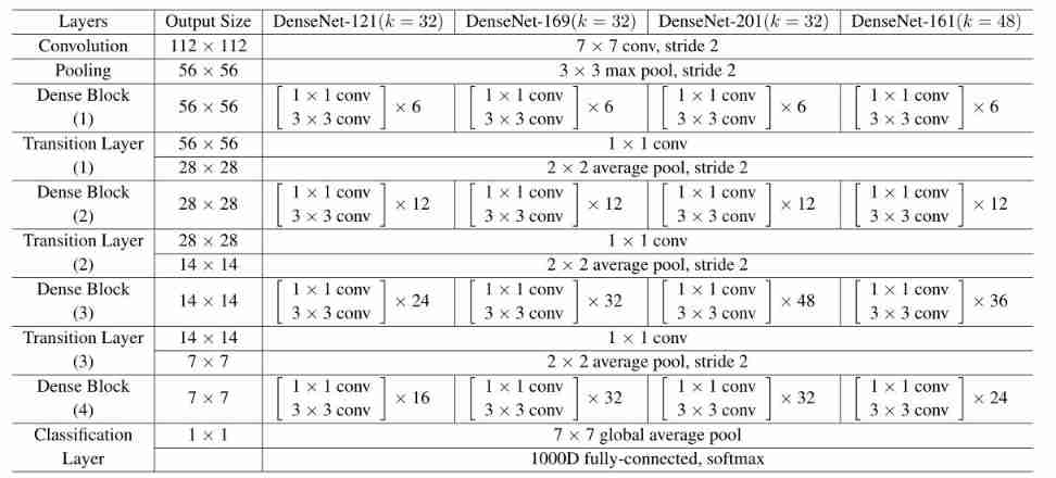
stay ImageNet The experiment on , stay $224\times 224$ The input image is used with 4 A dense block of DenseNet-BC structure . The initial convolution layer contains $2k$ Size is $7\times 7$ Convolution of , In steps of 2; The number of feature maps in all other layers also comes from the settings $k$. stay ImageNet The exact network configuration used on is shown in table 1 Shown .

surface 1：ImageNet Of DenseNet framework . front 3 The growth rate of networks is $k=32$, about DenseNet-161,$k=48$. Be careful , Each... Shown in the table “conv” Layer corresponds to BN-ReLU-Conv.

reference

[1] C. Cortes, X. Gonzalvo, V . Kuznetsov, M. Mohri, and S. Y ang. Adanet: Adaptive structural learning of artificial neural networks. arXiv preprint arXiv:1607.01097, 2016. 2

[3] S. E. Fahlman and C. Lebiere. The cascade-correlation learning architecture. In NIPS, 1989. 2

[9] B. Hariharan, P . Arbeláez, R. Girshick, and J. Malik. Hypercolumns for object segmentation and fine-grained localization. In CVPR, 2015. 2

[11] K. He, X. Zhang, S. Ren, and J. Sun. Deep residual learning for image recognition. In CVPR, 2016. 1, 2, 3, 4, 5, 6

[12] K. He, X. Zhang, S. Ren, and J. Sun. Identity mappings in deep residual networks. In ECCV, 2016. 2, 3, 5, 7

[23] J. Long, E. Shelhamer, and T. Darrell. Fully convolutional networks for semantic segmentation. In CVPR, 2015. 2

[30] P . Sermanet, K. Kavukcuoglu, S. Chintala, and Y . LeCun. Pedestrian detection with unsupervised multi-stage feature learning. In CVPR, 2013. 2

[36] C. Szegedy, V . V anhoucke, S. Ioffe, J. Shlens, and Z. Wojna. Rethinking the inception architecture for computer vision. In CVPR, 2016. 2, 3, 4

[37] S. Targ, D. Almeida, and K. Lyman. Resnet in resnet: Generalizing residual architectures. arXiv preprint arXiv:1603.08029, 2016. 2

[38] J. Wang, Z. Wei, T. Zhang, and W. Zeng. Deeply-fused nets. arXiv preprint arXiv:1605.07716, 2016. 3

[39] B. M. Wilamowski and H. Y u. Neural network learning without backpropagation. IEEE Transactions on Neural Networks, 21(11):1793–1803, 2010. 2

[40] S. Y ang and D. Ramanan. Multi-scale recognition with dagcnns. In ICCV, 2015. 2