[pytorch]fixmatch code explanation (super detailed)

The previous article talked about the process of data loading , This one goes further , Analyze how the training is conducted
Last link ： [pytorch]FixMatch Code details - Data loading

The mind map is linked below , The overall framework of the code is written in great detail
Mind mapping

Parameters default parameters

Data sets link
4000 A labeled dataset , That is, each class 400 Data with labels

I use the example given by the author by default for all parameters ：

python train.py --dataset cifar10 --num-labeled 4000 --arch wideresnet --batch-size 64 --lr 0.03 --expand-labels --seed 5 --out results/[email protected]4000.5

The values of each parameter in its runtime are as follows ：

INFO - __main__ -   {
    'T': 1, 'amp': False, 'arch': 'wideresnet', 'batch_size': 64, 'dataset': 'cifar10', 'device': device(type='cuda', index=0), 'ema_decay': 0.999, 'eval_step': 1024, 'expand_labels': True, 'gpu_id': 0, 'lambda_u': 1, 'local_rank': -1, 'lr': 0.03, 'mu': 7, 'n_gpu': 1, 'nesterov': True, 'no_progress': False, 'num_labeled': 4000, 'num_workers': 4, 'opt_level': 'O1', 'out': 'results/[email protected]', 'resume': '', 'seed': 5, 'start_epoch': 0, 'threshold': 0.95, 'total_steps': 1048576, 'use_ema': True, 'warmup': 0, 'wdecay': 0.0005, 'world_size': 1}

Then we bring these parameters into , See how each step works .

Data generation generate data

First , Is to generate an index of tagged and unlabeled data , Its presence cifar.py The code analysis in this document is shown in the previous chapter

base_dataset = datasets.CIFAR10(
        './CIFAR10', train=True, download=True)
labels = base_dataset.targets
label_per_class = 4000 // 10
labels = np.array(labels)
labeled_idx = []
# unlabeled data: all data (https://github.com/kekmodel/FixMatch-pytorch/issues/10)
unlabeled_idx = np.array(range(len(labels)))
for i in range(10):
    idx = np.where(labels == i)[0]
    idx = np.random.choice(idx, label_per_class, False)
    labeled_idx.extend(idx)
labeled_idx = np.array(labeled_idx)
print('number labeled_idx =',len(labeled_idx))
assert len(labeled_idx) == 4000

if True or 4000 < 64:
    num_expand_x = math.ceil(
        64 * 1024 / 4000)  #16.384 = 17
    labeled_idx = np.hstack([labeled_idx for _ in range(num_expand_x)])
np.random.shuffle(labeled_idx)
print('number labeled_idx = ',len(labeled_idx))
print('number unlabeled_idx =', len(unlabeled_idx))
train_labeled_idxs = labeled_idx
train_unlabeled_idxs = unlabeled_idx

give the result as follows , Unlabeled data uses all the data , The tagged data after data amplification is 68000 individual

number labeled_idx = 4000
number labeled_idx =  68000
number unlabeled_idx = 50000

Let's look at the changes in the picture
First , It is the original data image without any change ：

train_labeled_dataset = CIFAR10SSL(
        './data', train_labeled_idxs, train=True,
        transform=transforms.ToTensor())
train_iter = iter(train_labeled_dataset)

#  Visualization methods , Different picture data can be obtained by repeated execution 
imgs, label = next(train_iter)
print(image.size) # (32, 32)
image = transforms.ToPILImage()(imgs).convert('RGB')
image.show()
print(label)

then , We use changes without data enhancement , That is, the image change used by the author for the verification set . ToTensor() It's able to scale the grayscale from 0-255 Change to 0-1 Between , And then there's transform.Normalize() Then put 0-1 Change to (-1,1). Note that the size of the picture does not change , I just enlarged the picture when I took the screenshot .

cifar10_mean = (0.4914, 0.4822, 0.4465)
cifar10_std = (0.2471, 0.2435, 0.2616)
transform_val = transforms.Compose([
    transforms.ToTensor(),
    transforms.Normalize(mean=cifar10_mean, std=cifar10_std)])
train_labeled_dataset = CIFAR10SSL(
        './data', train_labeled_idxs, train=True,
        transform=transform_val)
train_iter = iter(train_labeled_dataset)

imgs, label = next(train_iter)
print(image.size) # (32, 32)
image = transforms.ToPILImage()(imgs).convert('RGB')
image.show()
print(label)

Then let's look at the data enhancement used for images with data （ two ）

cifar10_mean = (0.4914, 0.4822, 0.4465)
cifar10_std = (0.2471, 0.2435, 0.2616)
transform_labeled = transforms.Compose([
    transforms.RandomHorizontalFlip(), #Horizontally flip the given image randomly with a given probability.
    transforms.RandomCrop(size=32,
                          padding=int(32*0.125),
                          padding_mode='reflect'),
    transforms.ToTensor(),
    transforms.Normalize(mean=cifar10_mean, std=cifar10_std)
])
train_labeled_dataset = CIFAR10SSL(
        './data', train_labeled_idxs, train=True,
        transform=transform_labeled)
train_iter = iter(train_labeled_dataset)

imgs, label = next(train_iter)
print(image.size) # (32, 32)
image = transforms.ToPILImage()(imgs).convert('RGB')
image.show()
print(label) # 2 

For labels without data , We have two data enhancements , Weak enhancement and strong enhancement . Strong enhancement operation is described in this paper .

class TransformFixMatch(object):
    def __init__(self, mean, std):
        self.weak = transforms.Compose([
            transforms.RandomHorizontalFlip(),
            transforms.RandomCrop(size=32,
                                  padding=int(32*0.125),
                                  padding_mode='reflect')])
        self.strong = transforms.Compose([
            transforms.RandomHorizontalFlip(),
            transforms.RandomCrop(size=32,
                                  padding=int(32*0.125),
                                  padding_mode='reflect'),
            RandAugmentMC(n=2, m=10)])
        self.normalize = transforms.Compose([
            transforms.ToTensor(),
            transforms.Normalize(mean=mean, std=std)])

    def __call__(self, x):
        weak = self.weak(x)
        strong = self.strong(x)
        return self.normalize(weak), self.normalize(strong)
#  Enhanced operation . stay randaugment.py In file 
def fixmatch_augment_pool():
    # FixMatch paper
    augs = [(AutoContrast, None, None),
            (Brightness, 0.9, 0.05),
            (Color, 0.9, 0.05),
            (Contrast, 0.9, 0.05),
            (Equalize, None, None),
            (Identity, None, None),
            (Posterize, 4, 4),
            (Rotate, 30, 0),
            (Sharpness, 0.9, 0.05),
            (ShearX, 0.3, 0),
            (ShearY, 0.3, 0),
            (Solarize, 256, 0),
            (TranslateX, 0.3, 0),
            (TranslateY, 0.3, 0)]
    return augs
    
class RandAugmentMC(object):
    def __init__(self, n, m):
        assert n >= 1
        assert 1 <= m <= 10
        self.n = n
        self.m = m
        self.augment_pool = fixmatch_augment_pool()

    def __call__(self, img):
        ops = random.choices(self.augment_pool, k=self.n)
        for op, max_v, bias in ops:
            v = np.random.randint(1, self.m)
            if random.random() < 0.5:
                img = op(img, v=v, max_v=max_v, bias=bias)
        img = CutoutAbs(img, int(32*0.5))
        return img

cifar10_mean = (0.4914, 0.4822, 0.4465)
cifar10_std = (0.2471, 0.2435, 0.2616)

train_labeled_dataset = CIFAR10SSL(
        './data', train_labeled_idxs, train=True,
        transform=TransformFixMatch(mean=cifar10_mean, std=cifar10_std))
train_iter = iter(train_labeled_dataset)

(inputs_u_w, inputs_u_s), _ = next(train_iter)
print(inputs_u_s.size) # (32, 32)
image = transforms.ToPILImage()(inputs_u_s).convert('RGB')
image.show()

Weakly enhanced image results ( two ):

The result of strong reinforcement （ Run four times ）：

therefore , Generated with labels / Without a label / Verification set of dataset Class and dataloader as follows ：

labeled_dataset = CIFAR10SSL(
    './data', train_labeled_idxs, train=True,
    transform=transform_labeled)
# len = 68000
unlabeled_dataset = CIFAR10SSL(
    './data', train_unlabeled_idxs, train=True,
    transform=TransformFixMatch(mean=cifar10_mean, std=cifar10_std))
# len = 50000
test_dataset = datasets.CIFAR10(
    './data', train=False, transform=transform_val, download=False)
# len = 10000

train_sampler = RandomSampler
labeled_trainloader = DataLoader(
        labeled_dataset,
        sampler=train_sampler(labeled_dataset),
        batch_size=64,
        num_workers=4,
        drop_last=True)
# len = 6800/64 = 1062.5 （drop_last=True） = 1062 
unlabeled_trainloader = DataLoader(
    unlabeled_dataset,
    sampler=train_sampler(unlabeled_dataset),
    batch_size=64*7, # mu coefficient of unlabeled batch size  The super parameter in the original text μ 
    num_workers=4,
    drop_last=True)
# len = 50000/(64*7) = 111
test_loader = DataLoader(
    test_dataset,
    sampler=SequentialSampler(test_dataset),
    batch_size=64,
    num_workers=7)
# len = 10000/64 = 156.25（drop_last=False）= 157 

Build the model Build the model

def create_model():
    import models.wideresnet as models
    model = models.build_wideresnet(depth=28,
                                    widen_factor=2,
                                    dropout=0,
                                    num_classes=10)
    return model
    
model = create_model()
#print(model)
#for p in model.parameters():
# print(p.numel())
total_num = sum(p.numel() for p in model.parameters())
print(total_num) # 1467610  Total model parameters 

Training parameter setting Training parameter settings

When the parameter is set , There are many models for training tricks. Let me briefly talk about their settings . Here are some of the author's conclusions .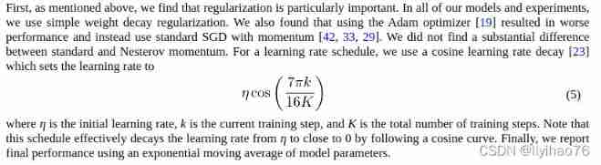

weight decay（ Weight attenuation ）

weight decay（ Weight attenuation ） The purpose is to prevent over fitting . In the loss function ,weight decay Is placed in the regular term （regularization） The previous coefficient , Regular terms generally indicate the complexity of the model , therefore weight decay The function of is to adjust the influence of model complexity on the loss function , if weight decay It's big , Then the value of the loss function of the complex model is large .
meanwhile , The author also mentioned the use of SGD Optimizer .

# weight decay default=5e-4
no_decay = ['bias', 'bn']
grouped_parameters = [
        {
    'params': [p for n, p in model.named_parameters() if not any(
            nd in n for nd in no_decay)], 'weight_decay': 5e-4},
        {
    'params': [p for n, p in model.named_parameters() if any(
            nd in n for nd in no_decay)], 'weight_decay': 0.0}
    ]
optimizer = optim.SGD(grouped_parameters, lr=0.03,
                      momentum=0.9, nesterov=True)

except bias and bn layer , Other layers use weight decay.

Learning rate decline （learning rate decay）

As the author mentioned in the original , For learning rate adjustment , We use cosine learning rate decay . At the same time Warmup operation . The learning rate was small at first , Upon reaching the set num_warmup_steps front , The learning rate is slowly increasing , Finally, the set learning rate is reached . after , Use cosine learning rate attenuation , The formula is as mentioned in the original text above .

def get_cosine_schedule_with_warmup(optimizer,
                                    num_warmup_steps,
                                    num_training_steps,
                                    num_cycles=7./16.,
                                    last_epoch=-1):
    def _lr_lambda(current_step):
        if current_step < num_warmup_steps:
            return float(current_step) / float(max(1, num_warmup_steps))
        no_progress = float(current_step - num_warmup_steps) / \
            float(max(1, num_training_steps - num_warmup_steps))
        return max(0., math.cos(math.pi * num_cycles * no_progress))

    return LambdaLR(optimizer, _lr_lambda, last_epoch)

scheduler = get_cosine_schedule_with_warmup(optimizer, 0, 2**20)

Learning rate is one of the most important super parameters in neural network training , There are many ways to optimize the learning rate ,Warmup It's one of them
( One )、 What is? Warmup?
Warmup Is in ResNet A method of preheating learning rate mentioned in the paper , It chooses to use a smaller learning rate at the beginning of training , Trained some epoches perhaps steps( such as 4 individual epoches,10000steps), Then modify it to the preset learning for training .

( Two )、 Why use Warmup?
Because at the beginning of training , Model weight (weights) It's randomly initialized , At this time, if you choose a larger learning rate , It may lead to the instability of the model ( Oscillate ), choice Warmup The way to warm up the learning rate , A few that can make you start training epoches Or some steps The internal learning rate is small , Under the preheating primary school attendance rate , The model can gradually become stable , After the model is relatively stable, select the preset learning rate for training , It makes the convergence speed of the model faster , The effect of the model is better .

ExampleExample：Resnet The paper uses a 110 Layer of ResNet stay cifar10 In training , First use 0.01 The learning rate is trained until the training error is less than 80%( Probably trained 400 individual steps), And then use 0.1 The learning rate of training .

Custom adjustments ： Custom adjust learning rate LambdaLR.
torch.optim.lr_scheduler.LambdaLR(optimizer, lr_lambda, last_epoch=-1, verbose=False)

Exponentially moving average （EMA）model

This algorithm is one of the most important algorithms currently in usage. From financial time series, signal processing to neural networks , it is being used quite extensively. Basically any data that is in a sequence.
We mostly use this algorithm to reduce the noise in noisy time-series data. The term we use for this is called “smoothing” the data.
The way we achieve this is by essentially weighing the number of observations and using their average. This is called as Moving Average.
In deep learning, the EMA (Exponential Moving Average) method is often used to average the parameters of the model in order to improve the test index and increase the robustness of the model.
In deep learning , Often use EMA（ Exponentially moving average ） This method averages the parameters of the model , In order to improve the test index and increase the model robustness .
I don't know much about this technique , You can read other people's articles ： 【 Alchemy skills 】 Exponentially moving average （EMA） The principle and PyTorch Realization

Training process training process

It's all in the notes , The process of each step is very clear

#  Get ready 
epochs = math.ceil(2**20/ 1024) #1024  total epoch
start_epoch = 0
test_accs = []
end = time.time() # Returns the timestamp of the current time 
def interleave(x, size):
    s = list(x.shape)
    return x.reshape([-1, size] + s[1:]).transpose(0, 1).reshape([-1] + s[1:])
def de_interleave(x, size):
    s = list(x.shape)
    return x.reshape([size, -1] + s[1:]).transpose(0, 1).reshape([-1] + s[1:])

labeled_iter = iter(labeled_trainloader)
unlabeled_iter = iter(unlabeled_trainloader)
model.train()
for epoch in range(start_epoch, epochs):
    #batch_time = AverageMeter()# It is only used to calculate and store some statistics , For example, statistics about losses .
    #data_time = AverageMeter()
    #losses = AverageMeter()
    #losses_x = AverageMeter()
    #losses_u = AverageMeter()
    #mask_probs = AverageMeter()
    p_bar = tqdm(range(1024))
    for batch_idx in range(1024):
        
        #  Use iter(next) Read the specified number of times batch, Not through Dataloader.Dataloader The length is also different .
        try:
            inputs_x, targets_x = labeled_iter.next()
            #print(inputs_x.shape) # torch.Size([64, 3, 32, 32])
            #print(targets_x.shape) # torch.Size([64])
            #print(targets_x)
        except:  #  When the loop ends , Start the cycle again 
            labeled_iter = iter(labeled_trainloader)
            inputs_x, targets_x = labeled_iter.next()
        try:
            (inputs_u_w, inputs_u_s), _ = unlabeled_iter.next()
            #print(inputs_u_w.shape) #torch.Size([448, 3, 32, 32])
            #print(inputs_u_s.shape) #torch.Size([448, 3, 32, 32])
        except:
            unlabeled_iter = iter(unlabeled_trainloader)
            (inputs_u_w, inputs_u_s), _ = unlabeled_iter.next()
        # print(time.time() - end) # data_time = 200 About seconds   Time to read a set of data 
        
        
        batch_size = inputs_x.shape[0] #64
        new_data = interleave(
                torch.cat((inputs_x, inputs_u_w, inputs_u_s)), 2*7+1) #'mu': 7
        # print(new_data.shape) torch.Size([960, 3, 32, 32]) 448+448+64 64*(2*7+1)  Merge data together 
        inputs = new_data.to(device)
        targets_x = targets_x.to(device)
        
        
        logits = model(inputs)
        #print(logits.shape) #torch.Size([960, 10])
        logits = de_interleave(logits, 2*7+1)
        #print(logits.shape) #torch.Size([960, 10])
        logits_x = logits[:batch_size]
        #print(logits_x.shape) #torch.Size([64, 10])
        logits_u_w, logits_u_s = logits[batch_size:].chunk(2)
        #print(logits_u_w.shape) #torch.Size([448, 10]) 
        
        # adopt weak_augment Sample calculation pseudo tag pseudo label and mask,
        # among ,mask It is used to filter which samples have the maximum prediction probability exceeding the threshold , It can be used , Which cannot be used 
        
        Lx = F.cross_entropy(logits_x, targets_x, reduction='mean') # With label data loss
        #print(Lx) # tensor(2.6575, device='cuda:0', grad_fn=<NllLossBackward0>)
        pseudo_label = torch.softmax(logits_u_w.detach()/1, dim=-1) # Output becomes probability 
        # pseudo label temperature = 1  The original softmax The function is T = 1 The special case of . 
        # T The higher the ,softmax Of output probability distribution The smoother , The greater the entropy of its distribution ,
        #  The information carried by the negative tag will be relatively enlarged , Model training will focus more on negative labels .
        max_probs, targets_u = torch.max(pseudo_label, dim=-1)
        #print(max_probs.shape) # torch.Size([448]) 448 Maximum probability value 
        #print(targets_u.shape) # torch.Size([448]) 448 Values of pseudo tags 
        #print(targets_u) #tensor([3, 5, 1 ....], device='cuda:0')
        mask = max_probs.ge(0.95).float() #'threshold': 0.95
        # torch.ge(a,b) Element by element comparison a,b Size 
        # print(mask.shape) #torch.Size([448]) 448 individual 0/1
        # print(F.cross_entropy(logits_u_s, targets_u,reduction='none')) # reduction='none' Not average , return 448 It's worth 
        Lu = (F.cross_entropy(logits_u_s, targets_u,
                                  reduction='none') * mask).mean() # Without label data loss, Among them through mask Conduct sample screening 
        #print(Lu) #tensor(0., device='cuda:0', grad_fn=<MeanBackward0>)
                
        loss = Lx + 1 * Lu # 'lambda_u': 1 # Complete loss function 
        
        
        print(time.time() - end) # 3439 second  batch_time  Time to calculate a set of data 
        end = time.time() # Prepare for the next round 
        print(mask.mean().item()) # mask_probs = mask The average of   Stands for more than threshold The proportion of the number of 

Running results result

First, let's take a look at the running results of the program
start

(torch) [email protected]-Precision-5820-Tower:~/LI/FixMatch-pytorch-master$ python train.py --dataset cifar10 --num-labeled 4000 --arch wideresnet --batch-size 64 --lr 0.03 --expand-labels --seed 5 --out results/test1
02/16/2022 17:48:12 - WARNING - __main__ -   Process rank: -1, device: cuda:0, n_gpu: 1, distributed training: False, 16-bits training: False
02/16/2022 17:48:12 - INFO - __main__ -   {
    'T': 1, 'amp': False, 'arch': 'wideresnet', 'batch_size': 64, 'dataset': 'cifar10', 'device': device(type='cuda', index=0), 'ema_decay': 0.999, 'eval_step': 1024, 'expand_labels': True, 'gpu_id': 0, 'lambda_u': 1, 'local_rank': -1, 'lr': 0.03, 'mu': 7, 'n_gpu': 1, 'nesterov': True, 'no_progress': False, 'num_labeled': 4000, 'num_workers': 4, 'opt_level': 'O1', 'out': 'results/test1', 'resume': '', 'seed': 5, 'start_epoch': 0, 'threshold': 0.95, 'total_steps': 1048576, 'use_ema': True, 'warmup': 0, 'wdecay': 0.0005, 'world_size': 1}
Files already downloaded and verified
02/16/2022 17:48:14 - INFO - models.wideresnet -   Model: WideResNet 28x2
02/16/2022 17:48:14 - INFO - __main__ -   Total params: 1.47M
02/16/2022 17:48:18 - INFO - __main__ -   ***** Running training *****
02/16/2022 17:48:18 - INFO - __main__ -     Task = [email protected]
02/16/2022 17:48:18 - INFO - __main__ -     Num Epochs = 1024
02/16/2022 17:48:18 - INFO - __main__ -     Batch size per GPU = 64
02/16/2022 17:48:18 - INFO - __main__ -     Total train batch size = 64
02/16/2022 17:48:18 - INFO - __main__ -     Total optimization steps = 1048576
Train Epoch: 1/1024. Iter: 1024/1024. LR: 0.0300. Data: 0.045s. Batch: 0.207s. Loss: 1.2336. Loss_x: 1.1920. Loss_u: 0.0416. Mask: 0.07. : 100%|█| 102
Test Iter:  157/ 157. Data: 0.005s. Batch: 0.012s. Loss: 1.8805. top1: 31.71. top5: 81.31. : 100%|██████████████████| 157/157 [00:02<00:00, 77.27it/s]
02/16/2022 17:51:52 - INFO - __main__ -   top-1 acc: 31.71
02/16/2022 17:51:52 - INFO - __main__ -   top-5 acc: 81.31
02/16/2022 17:51:52 - INFO - __main__ -   Best top-1 acc: 31.71
02/16/2022 17:51:52 - INFO - __main__ -   Mean top-1 acc: 31.71

Train Epoch: 2/1024. Iter: 1024/1024. LR: 0.0300. Data: 0.046s. Batch: 0.206s. Loss: 0.7871. Loss_x: 0.6212. Loss_u: 0.1659. Mask: 0.31. : 100%|█| 102
Test Iter:  157/ 157. Data: 0.005s. Batch: 0.012s. Loss: 0.9442. top1: 66.99. top5: 97.58. : 100%|██████████████████| 157/157 [00:01<00:00, 80.80it/s]
02/16/2022 17:55:22 - INFO - __main__ -   top-1 acc: 66.99
02/16/2022 17:55:22 - INFO - __main__ -   top-5 acc: 97.58
02/16/2022 17:55:22 - INFO - __main__ -   Best top-1 acc: 66.99
02/16/2022 17:55:22 - INFO - __main__ -   Mean top-1 acc: 49.35

Train Epoch: 3/1024. Iter: 1024/1024. LR: 0.0300. Data: 0.045s. Batch: 0.206s. Loss: 0.5908. Loss_x: 0.3215. Loss_u: 0.2692. Mask: 0.50. : 100%|█| 102
Test Iter:  157/ 157. Data: 0.005s. Batch: 0.012s. Loss: 0.6990. top1: 75.80. top5: 98.54. : 100%|██████████████████| 157/157 [00:02<00:00, 77.19it/s]
02/16/2022 17:58:53 - INFO - __main__ -   top-1 acc: 75.80
02/16/2022 17:58:53 - INFO - __main__ -   top-5 acc: 98.54
02/16/2022 17:58:54 - INFO - __main__ -   Best top-1 acc: 75.80
02/16/2022 17:58:54 - INFO - __main__ -   Mean top-1 acc: 58.17

It's running 100 Multiple epoch after

Train Epoch: 150/1024. Iter: 1024/1024. LR: 0.0294. Data: 0.017s. Batch: 0.157s. Loss: 0.2174. Loss_x: 0.0090. Loss_u: 0.2084. Mask: 0.90. : 100%|█| 1
Test Iter:  157/ 157. Data: 0.004s. Batch: 0.009s. Loss: 0.2418. top1: 94.17. top5: 99.87. : 100%|██████████████████| 157/157 [00:01<00:00, 99.77it/s]
02/17/2022 00:54:18 - INFO - __main__ -   top-1 acc: 94.17
02/17/2022 00:54:18 - INFO - __main__ -   top-5 acc: 99.87
02/17/2022 00:54:18 - INFO - __main__ -   Best top-1 acc: 94.28
02/17/2022 00:54:18 - INFO - __main__ -   Mean top-1 acc: 94.03

Train Epoch: 151/1024. Iter: 1024/1024. LR: 0.0294. Data: 0.018s. Batch: 0.158s. Loss: 0.2118. Loss_x: 0.0066. Loss_u: 0.2052. Mask: 0.90. : 100%|█| 1
Test Iter:  157/ 157. Data: 0.004s. Batch: 0.010s. Loss: 0.2393. top1: 94.37. top5: 99.91. : 100%|██████████████████| 157/157 [00:01<00:00, 89.00it/s]
02/17/2022 00:57:00 - INFO - __main__ -   top-1 acc: 94.37
02/17/2022 00:57:00 - INFO - __main__ -   top-5 acc: 99.91
02/17/2022 00:57:00 - INFO - __main__ -   Best top-1 acc: 94.37
02/17/2022 00:57:00 - INFO - __main__ -   Mean top-1 acc: 94.05

Train Epoch: 152/1024. Iter: 1024/1024. LR: 0.0294. Data: 0.017s. Batch: 0.158s. Loss: 0.2209. Loss_x: 0.0097. Loss_u: 0.2113. Mask: 0.90. : 100%|█| 1
Test Iter:  157/ 157. Data: 0.004s. Batch: 0.009s. Loss: 0.2414. top1: 94.19. top5: 99.86. : 100%|█████████████████| 157/157 [00:01<00:00, 100.27it/s]
02/17/2022 00:59:41 - INFO - __main__ -   top-1 acc: 94.19
02/17/2022 00:59:41 - INFO - __main__ -   top-5 acc: 99.86
02/17/2022 00:59:41 - INFO - __main__ -   Best top-1 acc: 94.37
02/17/2022 00:59:41 - INFO - __main__ -   Mean top-1 acc: 94.06

Train Epoch: 153/1024. Iter: 1024/1024. LR: 0.0294. Data: 0.017s. Batch: 0.159s. Loss: 0.2210. Loss_x: 0.0110. Loss_u: 0.2100. Mask: 0.90. : 100%|█| 1
Test Iter:  157/ 157. Data: 0.003s. Batch: 0.009s. Loss: 0.2439. top1: 94.07. top5: 99.87. : 100%|█████████████████| 157/157 [00:01<00:00, 101.27it/s]
02/17/2022 01:02:24 - INFO - __main__ -   top-1 acc: 94.07
02/17/2022 01:02:24 - INFO - __main__ -   top-5 acc: 99.87
02/17/2022 01:02:24 - INFO - __main__ -   Best top-1 acc: 94.37
02/17/2022 01:02:24 - INFO - __main__ -   Mean top-1 acc: 94.06

tensorboard See how the parameters change
Validation set parameter changes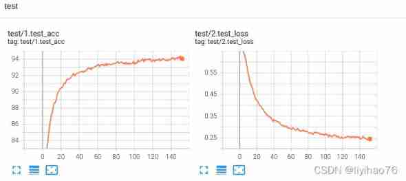

Parameter changes on the training set