当前位置:网站首页>Optimization cases of complex factor calculation: deep imbalance, buying and selling pressure index, volatility calculation
Optimization cases of complex factor calculation: deep imbalance, buying and selling pressure index, volatility calculation
2022-07-04 20:14:00 【51CTO】
In the data analysis work of the financial industry , The quality of data preprocessing and feature engineering often determines the actual effect of mathematical models .
Some financial indicators involve complex operations of high-dimensional and multi column in a large amount of original data , This will consume a lot of computing resources and development time .
This case is based on level2 Snapshot data , Developed 10 The depth of the minute frequency is unbalanced 、 Calculation script of buying and selling pressure index and volatility , For the purpose of DolphinDB Users provide reference examples when developing other similar factor calculation scripts , Improve development efficiency .
Calculation efficiency before and after optimization
- Total distributed table data :2,874,861,174
- The Shanghai 50 The data volume of the constituent stocks of the index :58,257,708
- The amount of data in the processed result table :267,490
Storage engine | Ten levels of trading volume and price storage | Calculation object | Logic CPU Check the number | Calculation time (s) |
OLAP | 40 Column | Column as unit | 8 | 450 |
OLAP | 40 Column | matrix | 8 | 450 |
TSDB | 40 Column | matrix | 8 | 27 |
TSDB | 4 Column | matrix | 8 | 25 |
1. Snapshot Data file structure
Field | meaning | Field | meaning | Field | meaning |
SecurityID | Stock code | LowPx | The lowest price | BidPrice[10] | Apply for ten prices |
DateTime | Date time | LastPx | The latest price | BidOrderQty[10] | Purchase ten quantities |
PreClosePx | Prec | TotalVolumeTrade | Total turnover | OfferPrice[10] | Apply for ten prices |
OpenPx | Starting price | TotalValueTrade | The total amount of the deal | OfferOrderQty[10] | Apply for ten sales |
HighPx | Highest price | InstrumentStatus | Transaction status | …… | …… |
The fields used in this case are Snapshot Some fields in , Include : Stock code 、 Snapshot time 、 Apply for ten prices , Purchase ten quantities , Apply for ten prices , Apply for ten sales .
The sample is 2020 Shanghai Stock Exchange 50 Index components :
- Stock code
       601318,600519,600036,600276,601166,600030,600887,600016,601328,601288,


600000,600585,601398,600031,601668,600048,601888,600837,601601,601012,


603259,601688,600309,601988,601211,600009,600104,600690,601818,600703,


600028,601088,600050,601628,601857,601186,600547,601989,601336,600196,


603993,601138,601066,601236,601319,603160,600588,601816,601658,600745
- 1.
- 2.
- 3.
- 4.
- 5.

- The name of the stock
        China safe 、 Guizhou Moutai 、 China Merchants Bank 、 Hengrui pharmaceutical 、 Societe generale 、 Citic securities, 、 Erie shares 、 Minsheng Bank 、 Bank of Communications 、 Agricultural bank of 、


 Pudong Development Bank 、 Conch Cement 、 Industrial and Commercial Bank of China 、 Sany heavy industry 、 Chinese architecture 、 Poly real estate 、 China free 、 Haitong securities 、 China Taibao 、 Longji shares 、


 wuxi 、 Huatai securities 、 Wanhua chemical 、 The bank of China, 、 Guotai junan 、 Shanghai Airport 、 Shanghai automotive industry corporation 、 Haier Zhijia 、 Everbright Bank 、 Three Ann photoelectric 、


 China petroleum & chemical corporation 、 China Shenhua 、 China Unicom 、 China life, 、 China's oil 、 China railway construction 、 Shandong gold 、 China heavy industries 、 Xinhua Insurance 、 Fosun medicine 、


 Luoyang molybdenum industry 、 Industrial wealth Federation 、 Citic built for 、 Hongta securities 、 China helped 、 Huiding Technology 、 UFIDA network 、 Beijing Shanghai High Speed Rail 、 Postal savings bank 、 Wentai technology
- 1.
- 2.
- 3.
- 4.
- 5.
2020 Shanghai Stock Exchange 14460 Securities Snapshot The data has been imported into DolphinDB In the database , It's about 28.75 Billion snapshot data , See Examples of importing domestic stock market data , altogether 174 Column .
2. Index definition
- Weighted Averaged Price(WAP): Weighted average price

- Depth Imbalance(DI): Depth imbalance

- Press: Buying and selling pressure index


Feature data resampling (10min window , And aggregate and calculate volatility )
Resampling utilization group by SecurityID, interval( TradeTime, 10m, "none" ) Method
- Realized Volatility(RV): Volatility is defined as the square root of the sum of squares of logarithmic returns
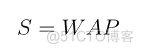
The price of the stock is always between the buying unit price and the selling unit price , Therefore, the weighted average price is used to replace the stock price in this project


3. SQL Optimize
Calculation of these indicators SQL The statement consists of the following parts :
The optimization part of this tutorial is the process of index calculation function .
3.1 Novice : Calculate in columns
Data use OLAP The storage engine stores .
Define the formula according to the index , Calculate in columns , Developers can quickly write the following SQL Code :
       /**


part1: Define calculation function


*/


def calPress(BidPrice0,BidPrice1,BidPrice2,BidPrice3,BidPrice4,BidPrice5,BidPrice6,BidPrice7,BidPrice8,BidPrice9,BidOrderQty0,BidOrderQty1,BidOrderQty2,BidOrderQty3,BidOrderQty4,BidOrderQty5,BidOrderQty6,BidOrderQty7,BidOrderQty8,BidOrderQty9,OfferPrice0,OfferPrice1,OfferPrice2,OfferPrice3,OfferPrice4,OfferPrice5,OfferPrice6,OfferPrice7,OfferPrice8,OfferPrice9,OfferOrderQty0,OfferOrderQty1,OfferOrderQty2,OfferOrderQty3,OfferOrderQty4,OfferOrderQty5,OfferOrderQty6,OfferOrderQty7,OfferOrderQty8,OfferOrderQty9){


  WAP = (BidPrice0*OfferOrderQty0+OfferPrice0*BidOrderQty0)\(BidOrderQty0+OfferOrderQty0)


  Bid_1_P_WAP_SUM = 1\(BidPrice0-WAP) + 1\(BidPrice1-WAP) + 1\(BidPrice2-WAP) + 1\(BidPrice3-WAP) + 1\(BidPrice4-WAP) + 1\(BidPrice5-WAP) + 1\(BidPrice6-WAP) + 1\(BidPrice7-WAP) + 1\(BidPrice8-WAP) + 1\(BidPrice9-WAP)


  Offer_1_P_WAP_SUM = 1\(OfferPrice0-WAP)+1\(OfferPrice1-WAP)+1\(OfferPrice2-WAP)+1\(OfferPrice3-WAP)+1\(OfferPrice4-WAP)+1\(OfferPrice5-WAP)+1\(OfferPrice6-WAP)+1\(OfferPrice7-WAP)+1\(OfferPrice8-WAP)+1\(OfferPrice9-WAP)


  BidPress = BidOrderQty0*((1\(BidPrice0-WAP))\Bid_1_P_WAP_SUM) + BidOrderQty1*((1\(BidPrice1-WAP))\Bid_1_P_WAP_SUM) + BidOrderQty2*((1\(BidPrice2-WAP))\Bid_1_P_WAP_SUM) + BidOrderQty3*((1\(BidPrice3-WAP))\Bid_1_P_WAP_SUM) + BidOrderQty4*((1\(BidPrice4-WAP))\Bid_1_P_WAP_SUM) + BidOrderQty5*((1\(BidPrice5-WAP))\Bid_1_P_WAP_SUM) + BidOrderQty6*((1\(BidPrice6-WAP))\Bid_1_P_WAP_SUM) + BidOrderQty7*((1\(BidPrice7-WAP))\Bid_1_P_WAP_SUM) + BidOrderQty8*((1\(BidPrice8-WAP))\Bid_1_P_WAP_SUM) + BidOrderQty9*((1\(BidPrice9-WAP))\Bid_1_P_WAP_SUM)


  OfferPress = OfferOrderQty0*((1\(OfferPrice0-WAP))\Offer_1_P_WAP_SUM) + OfferOrderQty1*((1\(OfferPrice1-WAP))\Offer_1_P_WAP_SUM) + OfferOrderQty2*((1\(OfferPrice2-WAP))\Offer_1_P_WAP_SUM) + OfferOrderQty3*((1\(OfferPrice3-WAP))\Offer_1_P_WAP_SUM) + OfferOrderQty4*((1\(OfferPrice4-WAP))\Offer_1_P_WAP_SUM) + OfferOrderQty5*((1\(OfferPrice5-WAP))\Offer_1_P_WAP_SUM) + OfferOrderQty6*((1\(OfferPrice6-WAP))\Offer_1_P_WAP_SUM) + OfferOrderQty7*((1\(OfferPrice7-WAP))\Offer_1_P_WAP_SUM) + OfferOrderQty8*((1\(OfferPrice8-WAP))\Offer_1_P_WAP_SUM) + OfferOrderQty9*((1\(OfferPrice9-WAP))\Offer_1_P_WAP_SUM)


  return log(BidPress)-log(OfferPress)


}


/**


part2: Define variables and assign values


*/


stockList=`601318`600519`600036`600276`601166`600030`600887`600016`601328`601288`600000`600585`601398`600031`601668`600048`601888`600837`601601`601012`603259`601688`600309`601988`601211`600009`600104`600690`601818`600703`600028`601088`600050`601628`601857`601186`600547`601989`601336`600196`603993`601138`601066`601236`601319`603160`600588`601816`601658`600745


dbName = "dfs://snapshot_SH_L2_OLAP"


tableName = "snapshot_SH_L2_OLAP"


snapshot = loadTable(dbName, tableName)


/**


part3: Execute SQL


*/


result = select


            avg((OfferPrice0\BidPrice0-1)) as BAS,


            avg((BidOrderQty0-OfferOrderQty0)\(BidOrderQty0+OfferOrderQty0)) as DI0,


            avg((BidOrderQty1-OfferOrderQty1)\(BidOrderQty1+OfferOrderQty1)) as DI1,


            avg((BidOrderQty2-OfferOrderQty2)\(BidOrderQty2+OfferOrderQty2)) as DI2,


            avg((BidOrderQty3-OfferOrderQty3)\(BidOrderQty3+OfferOrderQty3)) as DI3,


            avg((BidOrderQty4-OfferOrderQty4)\(BidOrderQty4+OfferOrderQty4)) as DI4,


            avg((BidOrderQty5-OfferOrderQty5)\(BidOrderQty5+OfferOrderQty5)) as DI5,


            avg((BidOrderQty6-OfferOrderQty6)\(BidOrderQty6+OfferOrderQty6)) as DI6,


            avg((BidOrderQty7-OfferOrderQty7)\(BidOrderQty7+OfferOrderQty7)) as DI7,


            avg((BidOrderQty8-OfferOrderQty8)\(BidOrderQty8+OfferOrderQty8)) as DI8,


            avg((BidOrderQty9-OfferOrderQty9)\(BidOrderQty9+OfferOrderQty9)) as DI9,


            avg(calPress(BidPrice0,BidPrice1,BidPrice2,BidPrice3,BidPrice4,BidPrice5,BidPrice6,BidPrice7,BidPrice8,BidPrice9, BidOrderQty0,BidOrderQty1,BidOrderQty2,BidOrderQty3,BidOrderQty4,BidOrderQty5,BidOrderQty6,BidOrderQty7,BidOrderQty8,BidOrderQty9,OfferPrice0,OfferPrice1,OfferPrice2,OfferPrice3,OfferPrice4,OfferPrice5,OfferPrice6,OfferPrice7,OfferPrice8,OfferPrice9,OfferOrderQty0,OfferOrderQty1,OfferOrderQty2,OfferOrderQty3,OfferOrderQty4,OfferOrderQty5,OfferOrderQty6,OfferOrderQty7,OfferOrderQty8,OfferOrderQty9)) as Press,


            sqrt(sum(pow((log((BidPrice0*OfferOrderQty0+OfferPrice0*BidOrderQty0)\(BidOrderQty0+OfferOrderQty0))-prev(log((BidPrice0*OfferOrderQty0+OfferPrice0*BidOrderQty0)\(BidOrderQty0+OfferOrderQty0)))),2))) as RV


    from snapshot


    where date(TradeTime) between 2020.01.01 : 2020.12.31, SecurityID in stockList, (time(TradeTime) between 09:30:00.000 : 11:29:59.999) || (time(TradeTime) between 13:00:00.000 : 14:56:59.999)


    group by SecurityID, interval( TradeTime, 10m, "none" ) as TradeTime
- 1.
- 2.
- 3.
- 4.
- 5.
- 6.
- 7.
- 8.
- 9.
- 10.
- 11.
- 12.
- 13.
- 14.
- 15.
- 16.
- 17.
- 18.
- 19.
- 20.
- 21.
- 22.
- 23.
- 24.
- 25.
- 26.
- 27.
- 28.
- 29.
- 30.
- 31.
- 32.
- 33.
- 34.
- 35.
- 36.
- 37.
- 38.
- 39.
- 40.
Above SQL in , involve BidPrice0-9、BidOrderQty0-9、OfferPrice0-9、OfferOrderQty0-9 common 40 Column data , And because the definition of indicators is more complex , Even after formula simplification , It is still difficult to solve the problem of lengthy code 、 Modify difficult problems .
Calculate the processing efficiency :
- Total distributed table data :2,874,861,174
- The Shanghai 50 The data volume of the constituent stocks of the index :58,257,708
- Logic CPU Check the number :8
- Average occupancy CPU The core number :4.5 individual
- Time consuming :450 second
3.2 Advanced : Splice the columns into a matrix for calculation
Data use OLAP The storage engine stores .
The above formula definitions are all calculations between columns , Actual calculations often occur in BidPrice,BidOrderQty,OfferPrice,OfferOrderQty this 4 Between large groups ( Each group 10 Column ), Therefore, these four groups can be regarded as n That's ok 10 Columns of the matrix . stay SQL In the middle of matrix Splicing , Then it is passed into the aggregate function for matrix operation , The sample code is as follows :
       /**


part1: Define calculation function


*/


defg featureEnginee(bidPrice,bidQty,offerPrice,offerQty){


  bas = offerPrice[0]\bidPrice[0]-1


  wap = (bidPrice[0]*offerQty[0] + offerPrice[0]*bidQty[0])\(bidQty[0]+offerQty[0])


  di = (bidQty-offerQty)\(bidQty+offerQty)


  bidw=(1.0\(bidPrice-wap))


  bidw=bidw\(bidw.rowSum())


  offerw=(1.0\(offerPrice-wap))


  offerw=offerw\(offerw.rowSum())


  press=log((bidQty*bidw).rowSum())-log((offerQty*offerw).rowSum())


  rv=sqrt(sum2(log(wap)-log(prev(wap))))


  return avg(bas),avg(di[0]),avg(di[1]),avg(di[2]),avg(di[3]),avg(di[4]),avg(di[5]),avg(di[6]),avg(di[7]),avg(di[8]),avg(di[9]),avg(press),rv


}


/**


part2: Define variables and assign values


*/


stockList=`601318`600519`600036`600276`601166`600030`600887`600016`601328`601288`600000`600585`601398`600031`601668`600048`601888`600837`601601`601012`603259`601688`600309`601988`601211`600009`600104`600690`601818`600703`600028`601088`600050`601628`601857`601186`600547`601989`601336`600196`603993`601138`601066`601236`601319`603160`600588`601816`601658`600745


dbName = "dfs://snapshot_SH_L2_OLAP"


tableName = "snapshot_SH_L2_OLAP"


snapshot = loadTable(dbName, tableName)


/**


part3: Execute SQL


*/


result1 = select


            featureEnginee(


            matrix(BidPrice0,BidPrice1,BidPrice2,BidPrice3,BidPrice4,BidPrice5,BidPrice6,BidPrice7,BidPrice8,BidPrice9),


            matrix(BidOrderQty0,BidOrderQty1,BidOrderQty2,BidOrderQty3,BidOrderQty4,BidOrderQty5,BidOrderQty6,BidOrderQty7, BidOrderQty8,BidOrderQty9),


            matrix(OfferPrice0,OfferPrice1,OfferPrice2,OfferPrice3,OfferPrice4,OfferPrice5,OfferPrice6,OfferPrice7,OfferPrice8, OfferPrice9),


            matrix(OfferOrderQty0,OfferOrderQty1,OfferOrderQty2,OfferOrderQty3,OfferOrderQty4,OfferOrderQty5,OfferOrderQty6, OfferOrderQty7,OfferOrderQty8,OfferOrderQty9)) as `BAS`DI0`DI1`DI2`DI3`DI4`DI5`DI6`DI7`DI8`DI9`Press`RV


    from snapshot


    where date(TradeTime) between 2020.01.01 : 2020.12.31, SecurityID in stockList, (time(TradeTime) between 09:30:00.000 : 11:29:59.999) || (time(TradeTime) between 13:00:00.000 : 14:56:59.999)


    group by SecurityID, interval( TradeTime, 10m, "none" ) as TradeTime map
- 1.
- 2.
- 3.
- 4.
- 5.
- 6.
- 7.
- 8.
- 9.
- 10.
- 11.
- 12.
- 13.
- 14.
- 15.
- 16.
- 17.
- 18.
- 19.
- 20.
- 21.
- 22.
- 23.
- 24.
- 25.
- 26.
- 27.
- 28.
- 29.
- 30.
- 31.
- 32.
- 33.
- 34.
- 35.
- 36.
 Through matrix processing , The code is greatly reduced , And the calculation code of the indicator formula can be easily seen in the user-defined aggregate function , This will greatly facilitate the subsequent modification of formula definitions and indicator calculation codes .
Calculate the processing efficiency :
- Total distributed table data :2,874,861,174
- The Shanghai 50 The data volume of the constituent stocks of the index :58,257,708
- Logic CPU Check the number :8
- Average occupancy CPU The core number :4.5 individual
- Time consuming :450 second
3.3 High performance 1:V2.00 Of TSDB Storage and Computing
DolphinDB V2.00 Added TSDB Storage engine , When creating partitioned databases and tables, it is associated with OLAP The storage engine differs in that it must specify engine and sortColumns, Create the statement as follows :
       dbName = "dfs://snapshot_SH_L2_TSDB"


tableName = "snapshot_SH_L2_TSDB"


dbTime = database(, VALUE, 2020.01.01..2020.12.31)


dbSymbol = database(, HASH, [SYMBOL, 20])


db = database(dbName, COMPO, [dbTime, dbSymbol], engine='TSDB')


createPartitionedTable(dbHandle=db, table=tbTemp, tableName=tableName, partitionColumns=`TradeTime`SecurityID, sortColumns=`SecurityID`TradeTime)
- 1.
- 2.
- 3.
- 4.
- 5.
- 6.
 Calculation code and 3.2 The advanced code is exactly the same .
because TSDB Query optimization of storage engine , Data computing performance has been greatly improved . Originally, it needs to run 450 Seconds to complete the calculation , After optimization, just run 27 second , Computing speed is not optimized code 17 times .
Calculate the processing efficiency :
- Total distributed table data :2,874,861,174
- The Shanghai 50 The data volume of the constituent stocks of the index :58,257,708
- Logic CPU Check the number :8
- Average occupancy CPU The core number :7.6 individual
- nothing level file index cache The calculation under takes time :27 second
- Yes level file index cache The calculation under takes time :16 second
3.4 High performance 2:V2.00 Of TSDB Use Array Vector Storage and Computing
DolphinDB from V2.00.4 Start , Storage support of distributed tables Array vector (array vector), Therefore, when storing data BidPrice0-9、BidOrderQty0-9、OfferPrice0-9、OfferOrderQty0-9 common 40 Column data in array vector The form is stored as BidPrice、BidOrderQty、OfferPrice、OfferOrderQty4 Column ,SQL The sample code of is as follows :
       /**


part1: Define calculation function


*/


defg featureEnginee(bidPrice,bidQty,offerPrice,offerQty){


  bas = offerPrice[0]\bidPrice[0]-1


  wap = (bidPrice[0]*offerQty[0] + offerPrice[0]*bidQty[0])\(bidQty[0]+offerQty[0])


  di = (bidQty-offerQty)\(bidQty+offerQty)


  bidw=(1.0\(bidPrice-wap))


  bidw=bidw\(bidw.rowSum())


  offerw=(1.0\(offerPrice-wap))


  offerw=offerw\(offerw.rowSum())


  press=log((bidQty*bidw).rowSum())-log((offerQty*offerw).rowSum())


  rv=sqrt(sum2(log(wap)-log(prev(wap))))


  return avg(bas),avg(di[0]),avg(di[1]),avg(di[2]),avg(di[3]),avg(di[4]),avg(di[5]),avg(di[6]),avg(di[7]),avg(di[8]),avg(di[9]),avg(press),rv


}


/**


part2: Define variables and assign values


*/


stockList=`601318`600519`600036`600276`601166`600030`600887`600016`601328`601288`600000`600585`601398`600031`601668`600048`601888`600837`601601`601012`603259`601688`600309`601988`601211`600009`600104`600690`601818`600703`600028`601088`600050`601628`601857`601186`600547`601989`601336`600196`603993`601138`601066`601236`601319`603160`600588`601816`601658`600745


dbName = "dfs://snapshot_SH_L2_TSDB_ArrayVector"


tableName = "snapshot_SH_L2_TSDB_ArrayVector"


snapshot = loadTable(dbName, tableName)


/**


part3: Execute SQL


*/


result = select


    featureEnginee(BidPrice,BidOrderQty,OfferPrice,OfferOrderQty) as `BAS`DI0`DI1`DI2`DI3`DI4`DI5`DI6`DI7`DI8`DI9`Press`RV


    from snapshot


    where date(TradeTime) between 2020.01.01 : 2020.12.31, SecurityID in stockList, (time(TradeTime) between 09:30:00.000 : 11:29:59.999) || (time(TradeTime) between 13:00:00.000 : 14:56:59.999)


    group by SecurityID, interval( TradeTime, 10m, "none" ) as TradeTime map
- 1.
- 2.
- 3.
- 4.
- 5.
- 6.
- 7.
- 8.
- 9.
- 10.
- 11.
- 12.
- 13.
- 14.
- 15.
- 16.
- 17.
- 18.
- 19.
- 20.
- 21.
- 22.
- 23.
- 24.
- 25.
- 26.
- 27.
- 28.
- 29.
- 30.
- 31.
- 32.
 Use TSDB Of array vector Data storage , Compare with in performance TSDB The improvement of the column storage is not obvious , But the code is simpler , It is convenient for later modification and maintenance .
Computational efficiency :
- Total distributed table data :2,874,861,174
- The Shanghai 50 The data volume of the constituent stocks of the index :58,257,708
- Logic CPU Check the number :8
- Average occupancy CPU The core number :7.6 individual
- nothing level file The calculation under the index cache takes time :25 second
- Yes level file The calculation under the index cache takes time :15 second
4. OLAP To TSDB Reasons for performance improvement
4.1 Database partition method
OLAP The code that the storage engine creates the partitioned database :
TSDB The code that the storage engine creates the partitioned database :
 DolphinDB The partition rules of are based on the database level , In this case ,OLAP Storage engine and TSDB The partition rules of the storage engine are the same , The first floor is divided by day , The second layer uses the hash algorithm to divide by the securities code 20 Districts . therefore ,14460 The daily data of securities are relatively evenly stored in 20 Within the divisions , The Shanghai 50 The data of index constituent stocks are also stored in multiple partitions ; Understand... From another angle , The same partition contains data of multiple securities with the same hash value .
stay DolphinDB in , Whether it's OLAP Storage engine or TSDB Storage engine , The idea of slicing data is consistent with the algorithm , So in this case , The only difference in the database creation code is ,TSDB The storage engine needs to specify parameters engine by TSDB, The default value of this parameter is OLAP.
4.2 Data table creation method
OLAP The code that the storage engine creates the partitioned data table :
 TSDB The code that the storage engine creates the partitioned data table :
 In the use of DolphinDB V2.00 TSDB Storage engine When creating a partitioned data table , Set up
 sortColumns=`SecurityID`TradeTime,sortColumns It usually consists of two parts :
-
sortKey: It can be composed of one or more query index columns , Time column without data - Time column : Time column in data , As a chronological sorting column of data in the partition
In this case ,sortKey=`SecurityID, Time is listed as TradeTime. And OLAP Compared with storage engine ,TSDB The same in each partition of the storage SecurityID The data of is continuous in the disk file , And in accordance with the TradeTime Strictly sort . Compared with OLAP Storage engine ,TSDB The storage engine is based on sortColumes When data filtering and querying fields , You can load only the data that meets the filtering conditions from the disk according to the index file in the partition .
The calculation sample of this case is 2020 Shanghai Stock Exchange 50 Index components , The calculation data source is 2020 Shanghai Stock Exchange 14460 All data of securities . If the OLAP Storage engine , We need to issue the certificate 50 The data of irrelevant securities in the partition involved in the index component stocks are loaded from disk to memory at the same time , Decompress the data 、 Filtering and calculation operations . If the TSDB, Only need to send the certificate 50 The data of index component stocks is loaded from disk into memory , Calculate the data .
4.3 OLAP Storage engine and TSDB Differences in storage engines
OLAP The storage engine maintains the order in which data is written , In one way append-only To store data on disk . Each column in each partition of the partition table is a file , For a column file , Multiple SecurityID The data of is added to the file according to the data writing order , So the same SecurityID The data of is very likely to be scattered in all positions of the whole column file . In this case , The query data table stores 14460 Data of securities , Although only the Shanghai Stock Exchange 50 Data of index constituent stocks , But in OLAP Under the storage engine , Will be Shanghai card 50 The data of irrelevant securities in the partition involved in the index component stocks are read from the disk to the memory at the same time for decompression , Reduce the efficiency of data extraction .
TSDB The storage engine is set sortColumns=`SecurityID`TradeTime, To the same SecurityID The storage of data is continuous , And the storage needs to be compressed :
- If the same
SecurityID All data is compressed together , Every time you query , Even if the data that really needs to be queried is just this SecurityID A small part of all data , You still need to read all the data from disk to memory for decompression , Reduce the efficiency of data reading . - TSDB The storage engine uses the same
SecurityID In the same LevelFile All the data in the are compressed and stored together , And specify a time interval for query , And the data in this time interval only occupy this SecurityID A small part of all the data . In this case , The same SecurityID According to sortColumns The last column TradeTime Sort , And split the data into a certain size ( The default is 16KB) A block of data (block) To store . While reading the data ,TSDB According to the filter conditions of the stock column and time column in the query statement, quickly locate the data block that meets the filter conditions , Then read these data blocks into memory and decompress , These data blocks usually account for only a small part of all data , This can greatly improve the efficiency of query .
4.4 Summary
In this case , Use TSDB Storage engine ratio OLAP The main reasons for the improvement of storage engine computing performance are as follows :
- In the calculation scenario of this case , The query data table stores the Shanghai Stock Exchange 2020 Of all securities in level2 Snapshot data ,14460 Securities in total 2,874,861,174 Data . The calculated sample data is 2020 Shanghai Stock Exchange 50 Index components , common 58,257,708 Data . Without any cache , And OLAP Compared with storage engine ,TSDB The storage engine only needs to read from the disk 58,257,708 Data .
- DolphinDB from V2.00.4 Start , Storage support of distributed tables Array vector (array vector), It is especially suitable for the storage of financial snapshot data and multi file volume and price data . For Shanghai Stock Exchange level2 Snapshot data , use array vector After storage , The compression ratio can be increased to 9~11. Without any cache , Compared with multi column storage , use TSDB Of array vector After storage , The number of data pieces read from the disk per unit time increases .
- level2 Many in snapshot data
- DolphinDB2.00TSDB Storage engine A... Is stored in a column and a row of the table vector object , So when doing matrix operation on multi grade volume and price data , The object returned by taking multiple rows of data in a column is a matrix , Compared with multi column storage , The process of matrix splicing is omitted .
5. summary
This case is based on the same calculation scenario , Developed 4 Share SQL Code :
- Novice Code data storage adopts DolphinDB Of OLAP Storage engine , Based on the idea of column calculation , The difficulty of code development is simple , But the code is verbose 、 Modify difficult problems , The calculation time is 450 second .
- Advanced Code data storage adopts DolphinDB Of OLAP Storage engine , Based on the idea of matrix calculation , The difficulty of code development is average , Less code , More clear expression of calculation logic , The calculation time is 450 second .
- High performance 1 piece Code data storage adopts DolphinDB Of TSDB Storage engine , Based on the idea of matrix calculation , The script code is exactly the same as the advanced code , nothing level file The calculation time under the index cache is 27 second , Yes level file The calculation time under the index cache is 16 second .
- High performance 2 piece Code data storage adopts DolphinDB Of TSDB Storage engine , And multi grade volume and price data adopt array vector For storage , Based on the idea of matrix calculation , Code reduction , It is convenient for later modification and maintenance , nothing level file The calculation time under the index cache is 25 second , Yes level file The calculation time under the index cache is 15 second .
For the purpose of DolphinDB Users provide reference examples when developing other similar factor calculation scripts , Improve development efficiency .
边栏推荐
- Functional interface
- Allure of pytest visual test report
- Kotlin condition control
- Development and construction of DFI ecological NFT mobile mining system
- Actual combat simulation │ JWT login authentication
- BCG 使用之CBCGPProgressDlgCtrl进度条使用
- 解密函数计算异步任务能力之「任务的状态及生命周期管理」
- 牛客小白月赛7 E Applese的超能力
- PHP pseudo original API docking method
- Basic use of kotlin
猜你喜欢
解密函数计算异步任务能力之「任务的状态及生命周期管理」
Detailed explanation of Audi EDI invoice message

On communication bus arbitration mechanism and network flow control from the perspective of real-time application
实战模拟│JWT 登录认证

Euler function
Siemens HMI download prompts lack of panel image solution
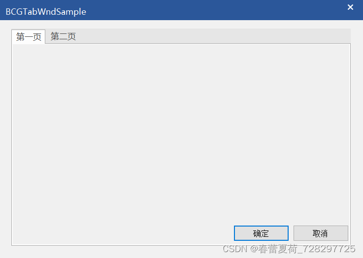
Cbcgptabwnd control used by BCG (equivalent to MFC TabControl)
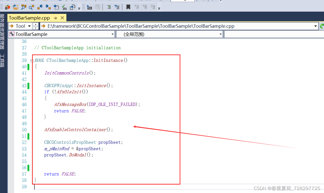
BCG 使用之新建向导效果
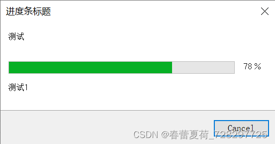
Cbcgpprogressdlg progress bar used by BCG

Development and construction of DFI ecological NFT mobile mining system
随机推荐
Informatics Olympiad 1336: [example 3-1] find roots and children
Pointnext: review pointnet through improved model training and scaling strategies++
Swagger suddenly went crazy
矩阵翻转(数组模拟)
1500万员工轻松管理,云原生数据库GaussDB让HR办公更高效
HDU 6440 2018 Chinese college student program design network competition
BCG 使用之CBCGPProgressDlg进度条使用
黑马程序员-软件测试--07阶段2-linux和数据库-09-24-linux命令学习步骤,通配符,绝对路径,相对路径,文件和目录常用命令,文件内容相关操作,查看日志文件,ping命令使用,
2022 Health Exhibition, health exhibition, Beijing Great Health Exhibition and health industry exhibition were held in November
C# 使用StopWatch测量程序运行时间
kotlin 继承
复杂因子计算优化案例:深度不平衡、买卖压力指标、波动率计算
Educational Codeforces Round 22 E. Army Creation
Niuke Xiaobai monthly race 7 I new Microsoft Office Word document
凌云出海记 | 沐融科技&华为云:打造非洲金融SaaS解决方案样板
Niuke Xiaobai month race 7 F question
HMM隐马尔可夫模型最详细讲解与代码实现
Anhui Zhong'an online culture and tourism channel launched a series of financial media products of "follow the small editor to visit Anhui"
1008 elevator (20 points) (PAT class a)
Cbcgptabwnd control used by BCG (equivalent to MFC TabControl)