【点云处理之论文狂读经典版14】—— Dynamic Graph CNN for Learning on Point Clouds

摘要

1. 背景： 对于计算机图形学中的许多应用而言，point clouds是一种灵活的几何表示，通常是大多数3D采集设备的原始输出
2. 问题： 尽管point clouds的hand-designed特征在很久以前就被提出来了，但是最近在image上很火的convolutional neural networks(CNNs)表明了将CNN应用到point clouds上的价值。Point clouds自身缺乏拓扑信息，所以需要设计一个可以恢复拓扑信息的模型，从而达到丰富point clouds表示能力的目的
3. 方法： 在CNN中嵌入了一个叫EdgeConv的模块
   • EdgeConv模块作用在graphs上，动态地对网络中每一层的graphs进行计算
   • EdgeConv模块可导，并且可以被嵌入任意现有的网络中
   • EdgeConv模块考虑了局部邻域信息和全局形状信息
   • EdgeConv 具有排序不变性
   • 特征空间中的multi-layer systems affinity采集了原始嵌入中潜在的长距离语义特征。
4. 代码：
   • TensorFlow版本
   • PyTorch版本

方法

• 为了挖掘局部几何结构，构造了一个局部邻域graph，并且在边上应用卷积操作，边连接着相邻的点对。
• 本文中的graph不固定，在网络的每一层都动态更新，也就是说，一个点的$kNN$集合中的元素在网络的层与层之间是变化的，是通过embeddings序列计算得到的。
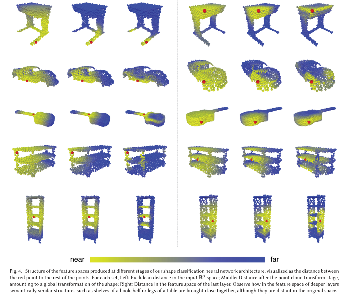
• 特征空间中的邻近性和输入不同，这样会导致信息在整个点云中的非局部扩散。

Edge Convolution

记$\mathbf{X}=\left\{{\mathbf{x}}_1,\dots ,{\mathbf{x}}_n\right\}\subseteq {\mathbb{R}}^F$为输入点云，其中$n$是点的数量，$F$是点的维度，在最简单的情况下，$F=3$，每个点都包括了3D坐标${\mathbf{x}}_i=\left(x_i,y_i,z_i\right)$，在其他情况下，还会包括颜色、法向量等，在网络的其他层，$F$表示点的特征维度。

我们计算一个有向图$\mathcal{G}=(\mathcal{V},\mathcal{E})$ ，表示局部点云结构，其中$\mathcal{V}=\{1,\dots ,n\}$， $\mathcal{E}\subseteq \mathcal{V}\times \mathcal{V}$分别是顶点和边。在最简单的情况下，构造一个$\mathrm{X}$的KNN graph $\mathcal{G}$。该graph包括self-loop，每个节点都会指向自己。定义边特征为${\mathbf{e}}_{ij}=h_{\Theta }\left({\mathbf{x}}_i,{\mathbf{x}}_j\right)$，其中$h_{\Theta }:{\mathbb{R}}^F\times$${\mathbb{R}}^F\to {\mathbb{R}}^{F^{\prime }}$是非线性函数，可学习参数为$\mathbf{\Theta }$。

最后，通过使用以channel为单位的对称聚合操作$\square$ (e.g., $\sum$ or max) 定义EdgeConv操作，在与从每个顶点发出的所有边缘相关联的边缘特征上进行聚合操作。在第$i$个顶点的EdgeConv输出表示为：
$${\mathbf{x}}_i^{\prime }=\underset{j:(i,j)\in \mathcal{E}}{\square }{h}_{\Theta }\left({\mathbf{x}}_i,{\mathbf{x}}_j\right)$$
其中${\mathbf{x}}_i$是central point，$\left\{{\mathbf{x}}_j:(i,j)\in \mathcal{E}\right\}$是${\mathbf{x}}_i$的neigboured points。总而言之，给定带有$n$个点的$F$维点云，EdgeConv会产生一个相同数量点的$F^{\prime }$维点云。

Choice of $h$ and $\square$

$h$的选择：

1. 卷积式：
   $$x_{im}^{\prime }=\sum _{j:(i,j)\in \mathcal{E}}{\mathbf{\theta }}_m\cdot {\mathbf{x}}_j.$$
   其中$\Theta =\left({\theta }_1,\dots ,{\theta }_M\right)$对$M$个不同的filters权值进行编码。每个${\theta }_m$都有着与$\mathbf{x}$相同的维度，$\cdot$表示内积。
2. PointNet式：
   $$h_{\Theta }\left({\mathbf{x}}_i,{\mathbf{x}}_j\right)=h_{\Theta }\left({\mathbf{x}}_i\right),$$
   只对全局形状信息编码，而不考虑局部邻域结构，算是EdgeConv的一种特殊情况。
3. Atzmon提出的PCNN式：
   $$x_{im}^{\prime }=\sum _{j\in \mathcal{V}}\left(h_{\mathbf{\theta }\left({\mathbf{x}}_j\right)}\right)g\left(u\left({\mathbf{x}}_i,{\mathbf{x}}_j\right)\right),$$
   其中 $g$是高斯kernel，$u$被用于计算欧式空间中的距离。
4. PointNet++式：
   $$h_{\mathbf{\Theta }}\left({\mathbf{x}}_i,{\mathbf{x}}_j\right)=h_{\mathbf{\Theta }}\left({\mathbf{x}}_j-{\mathbf{x}}_i\right).$$
   仅对局部信息进行编码，将整个形状划分为很多块，丢失了全局结构信息。
5. 本文使用的对称边函数：
   $$h_{\mathbf{\Theta }}\left({\mathbf{x}}_i,{\mathbf{x}}_j\right)={\bar{h}}_{\mathbf{\Theta }}\left({\mathbf{x}}_i,{\mathbf{x}}_j-{\mathbf{x}}_i\right).$$
   既结合了全局型状结构(通过以${\mathbf{x}}_i$为中心的坐标决定)，又考虑到了局部邻域信息(通过${\mathbf{x}}_j-{\mathbf{x}}_i$获取)。
   特别地，还可以通过下式表示EdgeConv的操作：
   $$e_{ijm}^{\prime }=\mathrm{ReLU}\left({\mathbf{\theta }}_m\cdot \left({\mathbf{x}}_j-{\mathbf{x}}_i\right)+{\mathbf{\varphi }}_m\cdot {\mathbf{x}}_i\right),$$
   然后再执行：
   $$x_{im}^{\prime }=\underset{j:(i,j)\in \mathcal{E}}{\max }{e}_{ijm}^{\prime },$$
   其中$\Theta =\left({\theta }_1,\dots ,{\theta }_M,{\varphi }_1,\dots ,{\varphi }_M\right)$。

$\square$选择为max

Dynamic Graph Update

我们的实验表明，利用每一层所产生的特征空间中的最近邻来重新计算graph是有用的。这是我们的方法与在固定输入graph上工作的graph CNN一个关键区别。这样的动态graph更新是我们的架构的名称DGCNN的原因。

在每一层，都有不同的graph ${\mathcal{G}}^{(l)}=\left({\mathcal{V}}^{(l)},{\mathcal{E}}^{(l)}\right)$，其中第$l$ 层的边的形式为$\left(i,j_{i1}\right),\dots ,\left(i,j_{i{k}_l}\right)$，也就是${\mathbf{x}}_{j_{i1}}^{(l)},\dots ,x_{j_{i{k}_l}}^{(l)}$是距离${\mathbf{x}}_i^{(l)}$最近的$k_l$个点。我们的网络学习如何构造每层中的graph $\mathcal{G}$，而不是在网络开始预测前就已经固定好了。在实现时，在距离空间中计算距离矩阵，然后对每个单点取最近的$k$个点。

Properties

Permutation Invariance

考虑到每一层的输出为：
$${\mathbf{x}}_i^{\prime }=\underset{j:(i,j)\in \mathcal{E}}{\max }{h}_{\mathbf{\Theta }}\left({\mathbf{x}}_i,{\mathbf{x}}_j\right),$$
由于max是一个对称函数，所以输出层${\mathrm{x}}_i^{\prime }$相对于输入 ${\mathbf{x}}_j$是排序不变的。全局最大池化操作对于聚合点特征也是排序不变的。

Translation Invariance

我们的操作有着一部分的translation invariance性质，因为边函数公式不受平移的影响，也可以选择性的受translation影响。考虑在点${\mathbf{x}}_j$和点${\mathbf{x}}_i$上进行平移，当平移 $T$时，有：
$$\begin{array}{rl}{e}_{ijm}^{\prime }& ={\mathbf{\theta }}_m\cdot \left({\mathbf{x}}_j+T-\left({\mathbf{x}}_i+T\right)\right)+{\mathbf{\varphi }}_m\cdot \left({\mathbf{x}}_i+T\right)\\ & ={\mathbf{\theta }}_m\cdot \left({\mathbf{x}}_j-{\mathbf{x}}_i\right)+{\mathbf{\varphi }}_m\cdot \left({\mathbf{x}}_i+T\right)\end{array}$$
如果令${\mathbf{\varphi }}_m=0$时，只考虑${\mathbf{x}}_j-{\mathbf{x}}_i$，那么该操作是完全平移不变的。但是模型会损失局部信息的获取，所以说还是部分translation invariance。

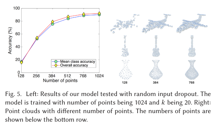
实验

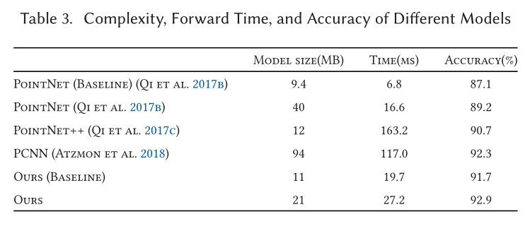
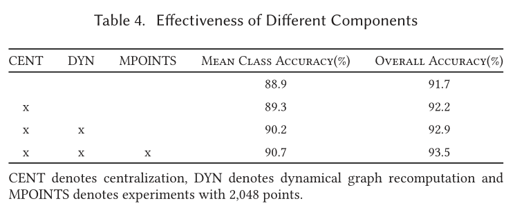
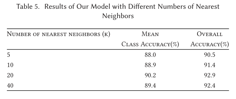
Classification

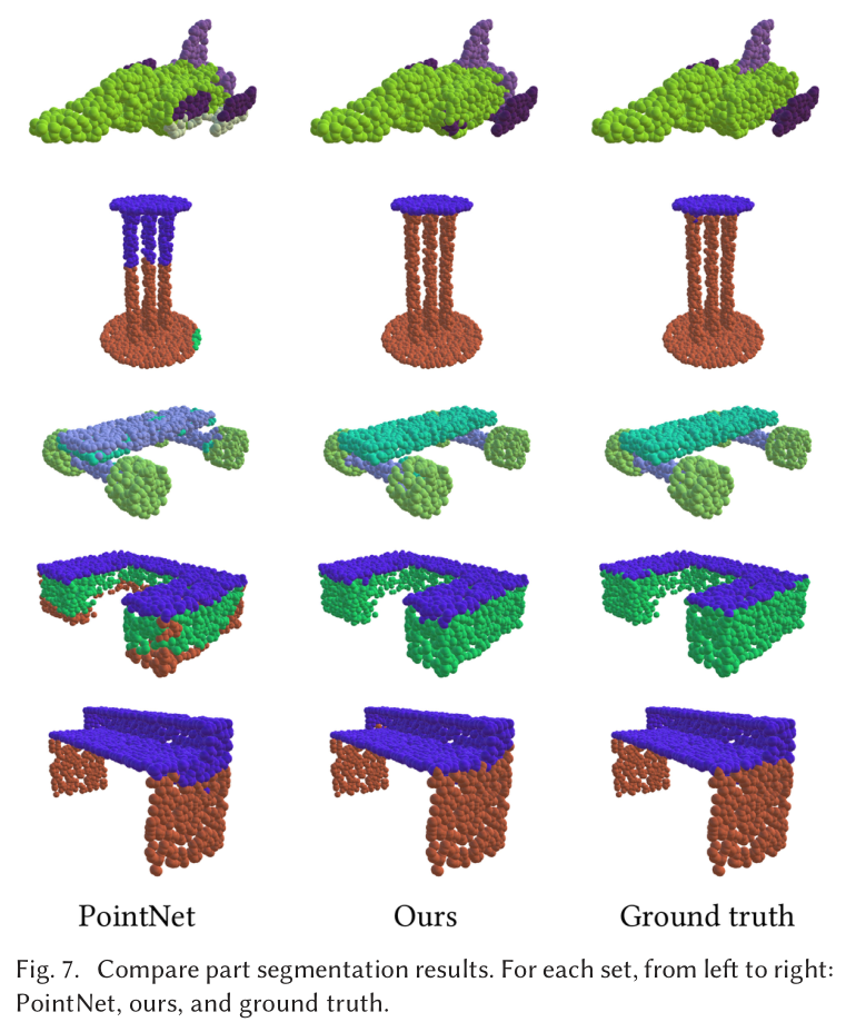
Part Segmentation

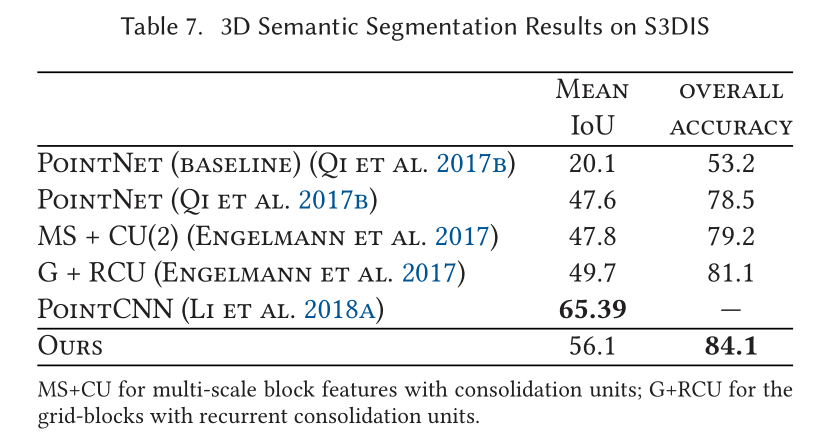
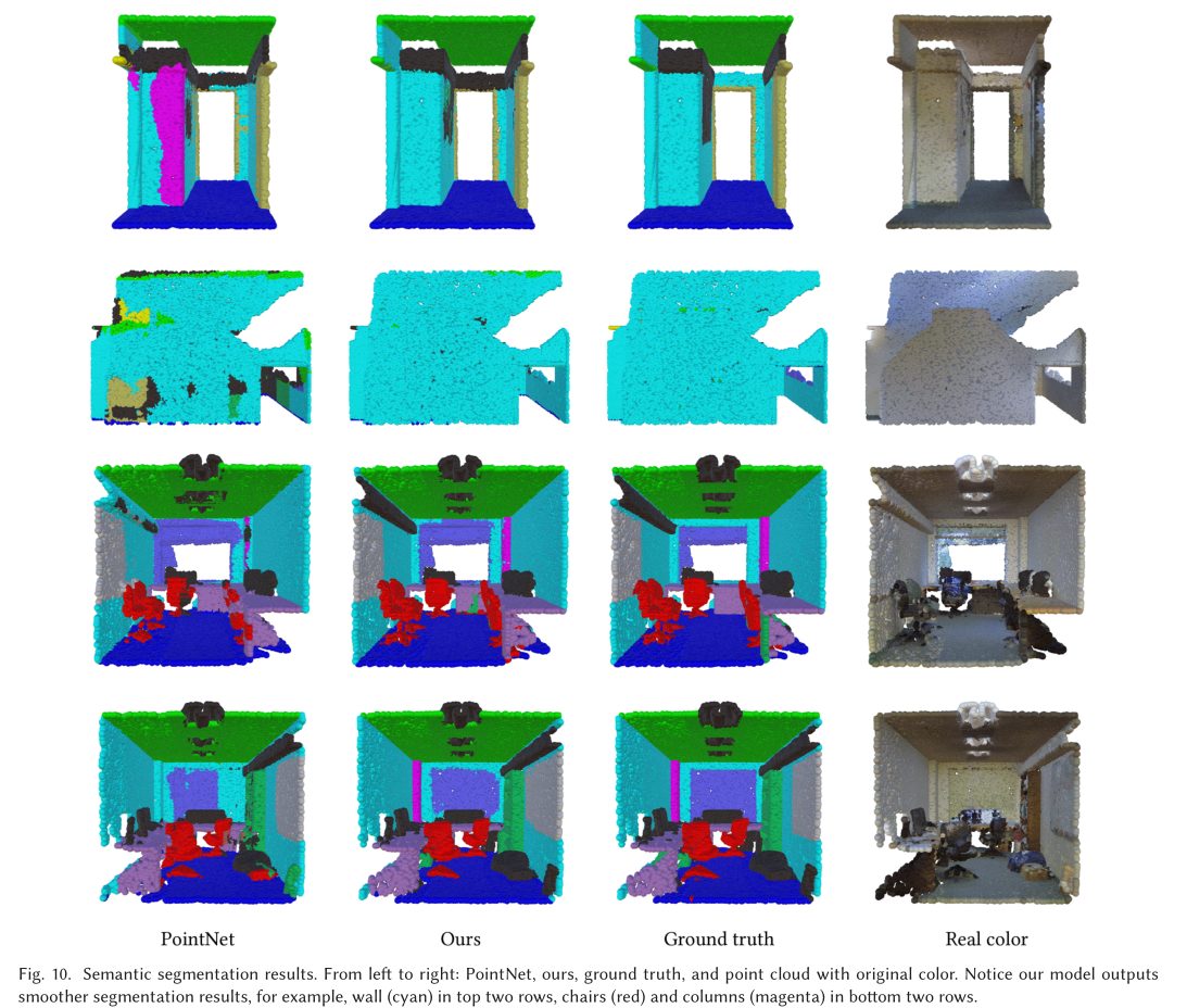
Indoor Scene Segmentation

展望

1. 通过结合更快的数据格式提高模型的速度，改用多元组，不去寻找点对之间的关系
2. 设计一个非共享的transformer网络，在每个local patch上都不同，更具灵活性

生词

1. dub v 被称为…
2. arguably adv 可以说是
3. emanate v 发出