当前位置:网站首页>CNN MNIST handwriting recognition
CNN MNIST handwriting recognition
2022-07-03 12:34:00 【kvnew】
#!/usr/bin/python3


from tensorflow.examples.tutorials.mnist import input_data
import tensorflow as tf
mnist = input_data.read_data_sets("MNIST_data/", one_hot=True)#  Read picture data set
sess = tf.InteractiveSession()#  establish session
#  One , Function declaration part


def weight_variable(shape):
    #  Normal distribution , The standard deviation is 0.1, Default maximum is 1, The minimum is -1, The mean for 0
    initial = tf.truncated_normal(shape, stddev=0.1)
    return tf.Variable(initial)
def bias_variable(shape):
    #  Create a structure for shape A matrix can also be said to be an array shape Declare its ranks , Initialize all values to 0.1
    initial = tf.constant(0.1, shape=shape)
    return tf.Variable(initial)
def conv2d(x, W):
    #  The number of convolution steps in each direction 1,SAME: Automatic filling outside the edge 0, Ergodic multiplication
    return tf.nn.conv2d(x, W, strides=[1, 1, 1, 1], padding='SAME')
def max_pool_2x2(x):
    #  Pooled convolution results (conv2d) The pool layer adopts kernel The size is 2*2, The number of steps is also 2, Peripheral supplement 0, Taking the maximum . The amount of data has shrunk 4 times
    return tf.nn.max_pool(x, ksize=[1, 2, 2, 1],strides=[1, 2, 2, 1], padding='SAME')


#  Two , Define the input / output structure


#  Declare a placeholder ,None Indicates that the number of input pictures is variable ,28*28 Image resolution
xs = tf.placeholder(tf.float32, [None, 28*28])
#  Category is 0-9 in total 10 Categories , Corresponding output classification result
ys = tf.placeholder(tf.float32, [None, 10])
keep_prob = tf.placeholder(tf.float32)
# x_image Also put xs reshape a 28*28*1 The shape of the , Because it's a gray picture , So the passage is 1. As a training input,-1 The number of pictures is variable
x_image = tf.reshape(xs, [-1, 28, 28, 1])


#  3、 ... and , Build network , Define the algorithm formula , That is to say forward The calculation of time


##  The first convolution operation  ##
#  The first and second parameters are the convolution kernel size , namely patch, The third parameter is the number of image channels , The fourth parameter is the number of convolution kernels , Represents how many convolution feature images will appear ;
W_conv1 = weight_variable([5, 5, 1, 32])
#  For each convolution kernel, there is a corresponding offset .
b_conv1 = bias_variable([32])
#  Multiply the picture by the convolution kernel , And add paranoia , Convolution results 28x28x32
h_conv1 = tf.nn.relu(conv2d(x_image, W_conv1) + b_conv1)
#  Pooling results 14x14x32  Multiply the convolution result by the pooled convolution kernel
h_pool1 = max_pool_2x2(h_conv1)


##  Second layer convolution operation  ##
# 32 Channel convolution , Convolution 64 Features
w_conv2 = weight_variable([5,5,32,64])
# 64 Paranoid data
b_conv2  = bias_variable([64])
#  Be careful h_pool1 It is the pool result of the upper layer ,# Convolution results 14x14x64
h_conv2 = tf.nn.relu(conv2d(h_pool1,w_conv2)+b_conv2)
#  Pooling results 7x7x64
h_pool2 = max_pool_2x2(h_conv2)
#  Original image size 28*28, The first image is reduced to 14*14, share 32 Zhang , After the second round, the image is reduced to 7*7, share 64 Zhang


##  Third layer full connection operation  ##
#  Two dimensional tensor , The first parameter 7*7*64 Of patch, It can also be thought that there is only one line 7*7*64 Convolution of data , The second parameter represents the total number of convolutions 1024 individual
W_fc1 = weight_variable([7*7*64, 1024])
# 1024 Paranoid data
b_fc1 = bias_variable([1024])
#  Pool the convolution result of the second layer reshape Cheng has only one line 7*7*64 Data # [n_samples, 7, 7, 64] ->> [n_samples, 7*7*64]
h_pool2_flat = tf.reshape(h_pool2, [-1, 7*7*64])
#  Convolution operation , The result is 1*1*1024, A single row multiplied by a single column equals 1*1 matrix ,matmul Realize the most basic matrix multiplication , differ tf.nn.conv2d Traversal multiplication of , It is automatically regarded as the forward vector and the backward vector
h_fc1 = tf.nn.relu(tf.matmul(h_pool2_flat, W_fc1) + b_fc1)


# dropout operation , Reduce overfitting , In fact, it is to reduce the weight of some inputs on the upper layer scale, Even set it to 0, Increase the weight of some inputs , Even set it to 2, Prevent the evaluation curve from shaking , I think it is necessary when there are few samples
#  Use placeholders , from dropout Automatically determine scale, You can also customize it , such as 0.5, according to tensorflow It can be seen from the documents , The actual value used in the program is 1/0.5=2, That is, some inputs are multiplied by 2, At the same time, some inputs are multiplied by 0
keep_prob = tf.placeholder(tf.float32)
h_fc1_drop = tf.nn.dropout(h_fc1,keep_prob) # Perform... On the convolution result dropout operation


##  Fourth layer output operation  ##
#  Two dimensional tensor ,1*1024 matrix convolution , common 10 A convolution , Corresponding to what we started ys The length is 10
W_fc2 = weight_variable([1024, 10])
b_fc2 = bias_variable([10])
#  The final classification , The result is 1*1*10 softmax and sigmoid It's all based on logistic Classification algorithm , One is multi classification, the other is two classification
y_conv=tf.nn.softmax(tf.matmul(h_fc1_drop, W_fc2) + b_fc2)


#  Four , Definition loss( Minimum error probability ), Select optimization optimization loss,
cross_entropy = -tf.reduce_sum(ys * tf.log(y_conv)) #  Define the cross entropy as loss function
train_step = tf.train.GradientDescentOptimizer(0.5).minimize(cross_entropy) #  Call the optimizer to optimize , In fact, it is through feeding data to win cross_entropy To minimize the


#  5、 ... and , Start data training and evaluation
correct_prediction = tf.equal(tf.argmax(y_conv,1), tf.argmax(ys,1))
accuracy = tf.reduce_mean(tf.cast(correct_prediction, tf.float32))
tf.global_variables_initializer().run()
for i in range(20000):
    batch = mnist.train.next_batch(50)
    if i%100 == 0:
        train_accuracy = accuracy.eval(feed_dict={x:batch[0], ys: batch[1], keep_prob: 1.0})
        print("step %d, training accuracy %g"%(i, train_accuracy))
    train_step.run(feed_dict={x: batch[0], ys: batch[1], keep_prob: 0.5})
print("test accuracy %g"%accuracy.eval(feed_dict={x: mnist.test.images, ys: mnist.test.labels, keep_prob: 1.0}))
边栏推荐
- (construction notes) ADT and OOP
- [combinatorics] permutation and combination (summary of permutation and combination content | selection problem | set permutation | set combination)
- 2.6 preliminary cognition of synergetic couroutines
- Is it safe to open an account for online stock speculation? Who can answer
- DEJA_ Vu3d - cesium feature set 053 underground mode effect
- LeetCode 0556. Next bigger element III - end of step 4
- Use of atomicinteger
- Official website of Unicode query
- 双链笔记·思源笔记综合评测:优点、缺点、评价
- MySQL time zone solution
猜你喜欢
![[official MySQL document] deadlock](/img/2d/04e97d696f20c2524701888ea9cd10.png)
[official MySQL document] deadlock

Flutter 退出登录二次确认怎么做才更优雅?
Basic knowledge of OpenGL (sort it out according to your own understanding)

Shutter: add gradient stroke to font
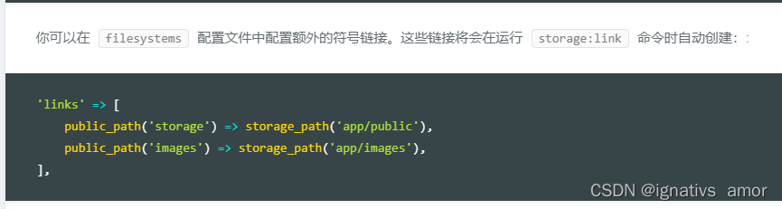
Symlink(): solution to protocol error in PHP artisan storage:link on win10

The future of cloud computing cloud native

Eureka self protection

Togaf certification self-study classic v2.0
LeetCode 0556.下一个更大元素 III - 4步讲完
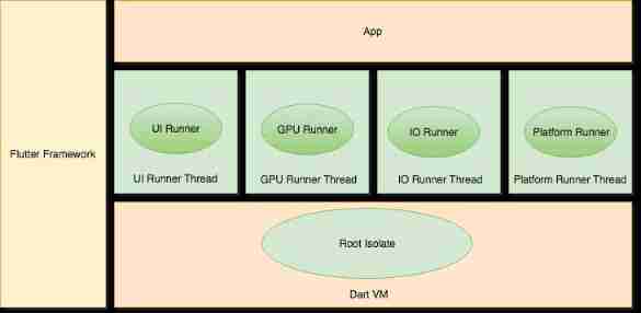
Fluent: Engine Architecture
随机推荐
Sword finger offer06 Print linked list from end to end
Shell: basic learning
Sword finger offer10- I. Fibonacci sequence
记录自己vulnhub闯关记录
(构造笔记)ADT与OOP
雲計算未來 — 雲原生
[combinatorics] permutation and combination (example of permutation and combination)
手机号码变成空号导致亚马逊账号登陆两步验证失败的恢复网址及方法
Applet wxss introduction
Apprendre à concevoir des entités logicielles réutilisables à partir de la classe, de l'API et du cadre
2020-09_ Shell Programming Notes
elastic_ L02_ install
temp
(构造笔记)GRASP学习心得
[download attached] password acquisition tool lazagne installation and use
【ManageEngine】IP地址扫描的作用
DEJA_ Vu3d - 054 of cesium feature set - simulate the whole process of rocket launch
257. All paths of binary tree
Lambda expression
[ManageEngine] the role of IP address scanning