当前位置:网站首页>[hard core dry goods] which company is better in data analysis? Choose pandas or SQL
[hard core dry goods] which company is better in data analysis? Choose pandas or SQL
2022-07-05 19:33:00 【Xinyi 2002】
Another week , Today, Xiaobian is going to talk about Pandas and SQL Grammatical differences between , I believe for many data analysts , Whether it's Pandas Module or SQL, They are all very many tools used in daily study and work , Of course, we can also be in Pandas From the module SQL sentence , By calling read_sql() Method
Want to get the source code of this tutorial , It can be answered in the background of official account 【20220704】 Can get
Building a database
First we pass SQL Statement is creating a new database , I'm sure everyone knows the basic grammar ,
CREATE TABLE  Table name  (
   Field name   data type  ...
)
Let's take a look at the specific code
import pandas as pd
import sqlite3
connector = sqlite3.connect('public.db')
my_cursor = connector.cursor()
my_cursor.executescript("""
CREATE TABLE sweets_types
(
    id integer NOT NULL,
    name character varying NOT NULL,
    PRIMARY KEY (id)
);
... Limited space , Refer to the source code for details ...
""")
At the same time, we also insert data into these new tables , The code is as follows
my_cursor.executescript("""
INSERT INTO sweets_types(name) VALUES
    ('waffles'),
    ('candy'),
    ('marmalade'),
    ('cookies'),
    ('chocolate');
... Limited space , Refer to the source code for details ...
""")
We can view the new table through the following code , And convert it to DataFrame Data set in format , The code is as follows
df_sweets = pd.read_sql("SELECT * FROM sweets;", connector)output

We have built a total of 5 Data sets , It mainly involves desserts 、 Types of desserts and data of processing and storage , For example, the data set of desserts mainly includes the weight of desserts 、 Sugar content 、 Production date and expiration time 、 Cost and other data , as well as
df_manufacturers = pd.read_sql("SELECT * FROM manufacturers", connector)output

The data set of processing involves the main person in charge and contact information of the factory , The warehouse data set involves the detailed address of the warehouse 、 City location, etc
df_storehouses = pd.read_sql("SELECT * FROM storehouses", connector)output

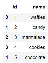
And the dessert category data set ,
df_sweets_types = pd.read_sql("SELECT * FROM sweets_types;", connector)output
Data screening
Screening of simple conditions
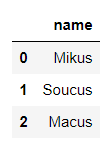
Next, let's do some data screening , For example, the weight of desserts is equal to 300 The name of dessert , stay Pandas The code in the module looks like this
#  Convert data type
df_sweets['weight'] = pd.to_numeric(df_sweets['weight'])
#  Output results
df_sweets[df_sweets.weight == 300].name
output
1      Mikus
6     Soucus
11     Macus
Name: name, dtype: object
Of course, we can also pass pandas In the middle of read_sql() Method to call SQL sentence
pd.read_sql("SELECT name FROM sweets WHERE weight = '300'", connector)output
Let's look at a similar case , The screening cost is equal to 100 The name of dessert , The code is as follows
# Pandas
df_sweets['cost'] = pd.to_numeric(df_sweets['cost'])
df_sweets[df_sweets.cost == 100].name

# SQL
pd.read_sql("SELECT name FROM sweets WHERE cost = '100'", connector)
output
MiltyFor text data , We can also further screen out the data we want , The code is as follows
# Pandas
df_sweets[df_sweets.name.str.startswith('M')].name

# SQL
pd.read_sql("SELECT name FROM sweets WHERE name LIKE 'M%'", connector)
output
Milty
Mikus
Mivi
Mi
Misa
Maltik
Macus
Of course. SQL Wildcards in statements ,% Means to match any number of letters , and _ Means to match any letter , The specific differences are as follows
# SQL
pd.read_sql("SELECT name FROM sweets WHERE name LIKE 'M%'", connector)
output
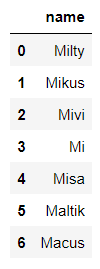
pd.read_sql("SELECT name FROM sweets WHERE name LIKE 'M_'", connector)output

Screening of complex conditions
Let's take a look at data filtering with multiple conditions , For example, we want the weight to be equal to 300 And the cost price is controlled at 150 The name of dessert , The code is as follows
# Pandas
df_sweets[(df_sweets.cost == 150) & (df_sweets.weight == 300)].name

# SQL
pd.read_sql("SELECT name FROM sweets WHERE cost = '150' AND weight = '300'", connector)
output
MikusOr the cost price can be controlled within 200-300 Dessert name between , The code is as follows
# Pandas
df_sweets[df_sweets['cost'].between(200, 300)].name

# SQL
pd.read_sql("SELECT name FROM sweets WHERE cost BETWEEN '200' AND '300'", connector)
output

If it comes to sorting , stay SQL It uses ORDER BY sentence , The code is as follows
# SQL
pd.read_sql("SELECT name FROM sweets ORDER BY id DESC", connector)
output

And in the Pandas What is called in the module is sort_values() Method , The code is as follows
# Pandas
df_sweets.sort_values(by='id', ascending=False).name
output
11     Macus
10    Maltik
9        Sor
8         Co
7     Soviet
6     Soucus
5     Soltic
4       Misa
3         Mi
2       Mivi
1      Mikus
0      Milty
Name: name, dtype: object
Select the dessert name with the highest cost price , stay Pandas The code in the module looks like this
df_sweets[df_sweets.cost == df_sweets.cost.max()].nameoutput
11    Macus
Name: name, dtype: object
And in the SQL The code in the statement , We need to first screen out which dessert is the most expensive , Then proceed with further processing , The code is as follows
pd.read_sql("SELECT name FROM sweets WHERE cost = (SELECT MAX(cost) FROM sweets)", connector) We want to see which cities are warehousing , stay Pandas The code in the module looks like this , By calling unique() Method
df_storehouses['city'].unique()output
array(['Moscow', 'Saint-petersburg', 'Yekaterinburg'], dtype=object) And in the SQL The corresponding sentence is DISTINCT keyword
pd.read_sql("SELECT DISTINCT city FROM storehouses", connector)Data grouping Statistics
stay Pandas Group statistics in modules generally call groupby() Method , Then add a statistical function later , For example, it is to calculate the mean value of scores mean() Method , Or summative sum() Methods, etc. , For example, we want to find out the names of desserts produced and processed in more than one city , The code is as follows
df_manufacturers.groupby('name').name.count()[df_manufacturers.groupby('name').name.count() > 1]output
name
Mishan    2
Name: name, dtype: int64
And in the SQL The grouping in the statement is also GROUP BY, If there are other conditions later , It's using HAVING keyword , The code is as follows
pd.read_sql("""
SELECT name, COUNT(name) as 'name_count' FROM manufacturers
GROUP BY name HAVING COUNT(name) > 1
""", connector)
Data merging
When two or more datasets need to be merged , stay Pandas Modules , We can call merge() Method , For example, we will df_sweets Data set and df_sweets_types Merge the two data sets , among df_sweets In the middle of sweets_types_id Is the foreign key of the table
df_sweets.head()output

df_sweets_types.head()output

The specific data consolidation code is as follows
df_sweets_1 = df_sweets.merge(df_sweets_types, left_on='sweets_types_id', right_on='id')output
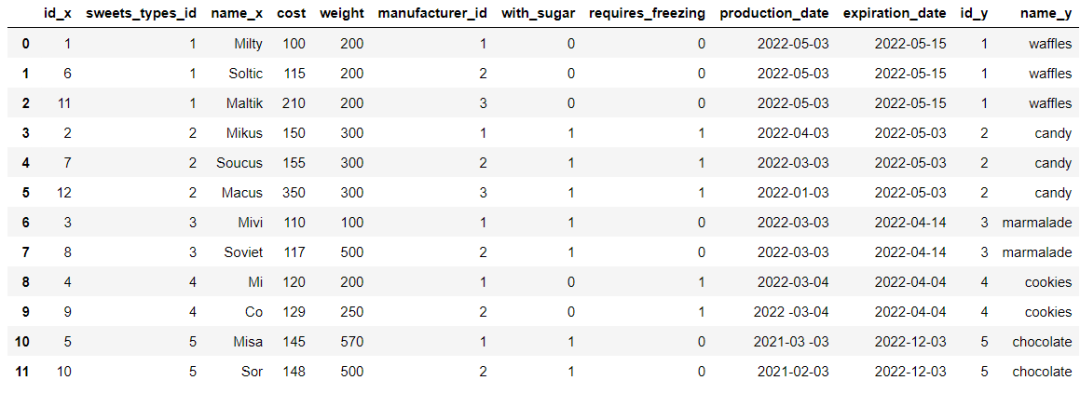
We will further screen out chocolate flavored desserts , The code is as follows
df_sweets_1.query('name_y == "chocolate"').name_xoutput
10    Misa
11     Sor
Name: name_x, dtype: object
and SQL The sentence is relatively simple , The code is as follows
# SQL
pd.read_sql("""
SELECT sweets.name FROM sweets
JOIN sweets_types ON sweets.sweets_types_id = sweets_types.id
WHERE sweets_types.name = 'chocolate';
""", connector)
output

The structure of the data set
Let's take a look at the structure of the data set , stay Pandas View directly in the module shape Attribute is enough , The code is as follows
df_sweets.shapeoutput
(12, 10) And in the SQL In the sentence , It is
pd.read_sql("SELECT count(*) FROM sweets;", connector)output

NO.1
Previous recommendation
Historical articles
8 Cool visual charts , Quickly write the visual analysis report that the boss likes to see
【 Hard core dry goods 】Pandas Data type conversion in modules
use Python among Plotly.Express The module draws several charts , I was really amazed !!
Share 、 Collection 、 give the thumbs-up 、 I'm looking at the arrangement ?


边栏推荐
- 【obs】libobs-winrt :CreateDispatcherQueueController
- JAD的安装、配置及集成IDEA
- webuploader文件上传 拖拽上传 进度监听 类型控制 上传结果监听控件
- MMO项目学习一:预热
- 关于 Notion-Like 工具的反思和畅想
- shell编程基础(第9篇:循环)
- 如何实现游戏中的在线计时器和离线计时器
- Android面试,android音视频开发
- Ten years at sea: old and new relay, dark horse rising
- What does software testing do? What are the requirements for learning?
猜你喜欢
Teach you to deal with JS reverse picture camouflage hand in hand

Debezium系列之:记录mariadb数据库删除多张临时表debezium解析到的消息以及解决方法
HiEngine:可媲美本地的云原生内存数据库引擎
Webuploader file upload drag upload progress monitoring type control upload result monitoring control
Mysql如何对json数据进行查询及修改
Apprentissage du projet MMO I: préchauffage
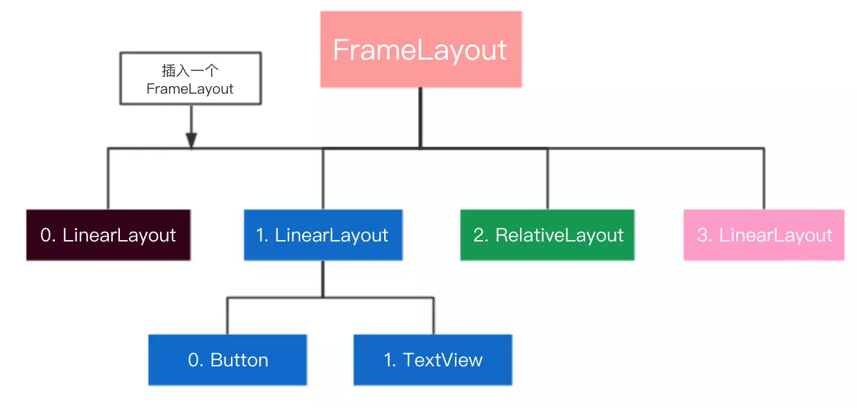
大厂面试必备技能,2022Android不死我不倒

测试外包公司怎么样?
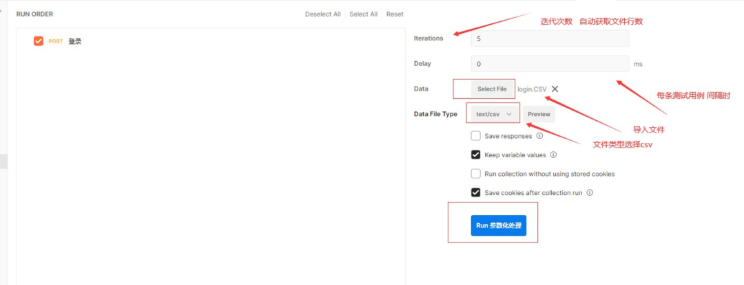
Postman core function analysis - parameterization and test report
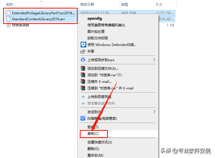
Tutoriel de téléchargement et d'installation du progiciel fuzor 2020
随机推荐
JAD的安装、配置及集成IDEA
Xaas trap: all things serve (possible) is not what it really needs
Do you know several assertion methods commonly used by JMeter?
JS solution force deduction daily question (12) - 556 Next larger element III (2022-7-3)
#夏日挑战赛#数据库学霸笔记,考试/面试快速复习~
S7-200SMART利用V90 MODBUS通信控制库控制V90伺服的具体方法和步骤
Debezium系列之:postgresql从偏移量加载正确的最后一次提交 LSN
Oracle故障处理:Ora-10873:file * needs to be either taken out of backup or media recovered
Debezium系列之:记录mariadb数据库删除多张临时表debezium解析到的消息以及解决方法
PHP利用ueditor实现上传图片添加水印
Go语言 | 03 数组、指针、切片用法
软件测试工程师是做什么的?待遇前景怎么样?
The relationship between temperature measurement and imaging accuracy of ifd-x micro infrared imager (module)
How to apply smart contracts more wisely in 2022?
【C语言】字符串函数及模拟实现strlen&&strcpy&&strcat&&strcmp
flume系列之:拦截器过滤数据
The basic grammatical structure of C language
Which securities company is better and which platform is safer for mobile account opening
What are the reliable domestic low code development platforms?
安卓面试宝典,2022Android面试笔试总结
