[mathematics] [continuum mechanics] symmetry tensor, strain tensor and stress tensor in fluid mechanics

The origin of the problem

stay splishsplash Thesis tutorial among , When it comes to stickiness , There is such a page PPT

This is the basic knowledge of fluid mechanics , That is, it is constructed by Newton constitutive model NS equation .

Let's first look at the formula on the left

It is called Cauchy momentum equation . This equation is applicable to both fluid mechanics and solid mechanics . Therefore, it can be regarded as NS The existence of more fundamental equations . It's actually a linear momentum equation . The acceleration on the left , On the right is internal power （ Expressed by stress , Is surface force ） And external forces （ Usually physical strength ）.

among T It's the stress tensor .

Let's look at the formula on the right .

This formula is Newton's constitutive equation . Equations constructed for Newtonian fluids . If it wasn't Newtonian fluid , Not applicable . The so-called constitutive equation , Is to find the relationship between stress and strain . actually , In terms of Solid Mechanics , The second equation is a geometric equation . The first equation is the physical equation , Or constitutive equation . We don't distinguish between , It's called his constitutive equation .

however , Our focus is not on the equation itself . Our aim is to make readers Be familiar with these mathematical signs The meaning of . in other words , We from Tensor mathematics Look at these quantities from the angle of What is the form of a matrix that we are familiar with ？

Nothing else is difficult . The only thing we are not familiar with is the velocity gradient . namely
$$\nabla \mathbf{v}$$

We previously wrote a popular introduction to tensors , as follows ：
https://blog.csdn.net/weixin_43940314/article/details/123559800

velocity gradient

Velocity is obviously a vector
$$\mathbf{v}=(u,v,w{)}^T$$

and nabla The operator is just a vector
$$\nabla =(\frac{\partial }{\partial x},\frac{\partial }{\partial y},\frac{\partial }{\partial z}{)}^T$$

Vector and vector write together , There is no sign in the middle , It's actually a multiplication of （ Also called dyadic ）. Sometimes we take the initiative to add a symbol , It's written in $⨂$.

Actually , gradient Namely nabla Multiplication of operators and physical quantities .

What rule does the multiplication follow ？

Union multiplication and dot multiplication 、 Cross multiplication is different , It does nothing ！ Just simply write the vectors side by side .

Besides , remember ： And multiplication is ascending , The order of the result is to add up the original order ！

Let's write the union multiplication in the familiar matrix form .

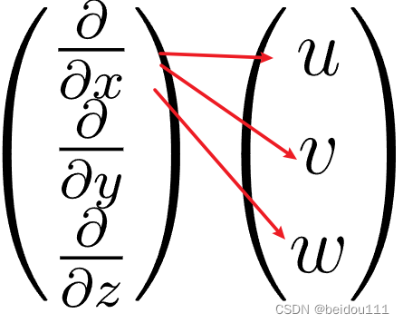
We write line by line
$$\nabla \otimes \mathbf{v}=\left(\begin{array}{c}\frac{\partial }{\partial x}\\ \frac{\partial }{\partial y}\\ \frac{\partial }{\partial z}\end{array}\right)\otimes \left(\begin{array}{c}u\\ v\\ w\end{array}\right)$$

1 first line

The corresponding items are simply written side by side

1.1 Component and form

Write in the form of component sum
$$\frac{\partial u}{\partial x}\mathbf{i}\mathbf{i}+\frac{\partial v}{\partial x}\mathbf{i}\mathbf{j}+\frac{\partial w}{\partial x}\mathbf{i}\mathbf{k}$$

1.2 Matrix form

Or in the form of a matrix

That is to say

$$\left(\begin{array}{ccc}\frac{\partial u}{\partial x}& \frac{\partial v}{\partial x}& \frac{\partial w}{\partial x}\\ \cdots & \cdots & \cdots \\ \cdots & \cdots & \cdots \end{array}\right)$$

2 The second line

Empathy

2.1 Component and form

Write in the form of component sum
$$\frac{\partial u}{\partial y}\mathbf{i}\mathbf{i}+\frac{\partial v}{\partial y}\mathbf{i}\mathbf{j}+\frac{\partial w}{\partial y}\mathbf{i}\mathbf{k}$$

2.2 Matrix form

Or in the form of a matrix

That is to say

$$\left(\begin{array}{ccc}\cdots & \cdots & \cdots \\ \frac{\partial u}{\partial y}& \frac{\partial v}{\partial y}& \frac{\partial w}{\partial y}\\ \cdots & \cdots & \cdots \end{array}\right)$$

3 The third line

Empathy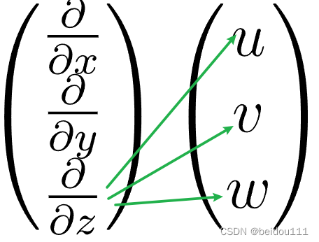

3.1 Component and form

Write in the form of component sum
$$\frac{\partial u}{\partial z}\mathbf{i}\mathbf{i}+\frac{\partial v}{\partial z}\mathbf{i}\mathbf{j}+\frac{\partial w}{\partial z}\mathbf{i}\mathbf{k}$$

3.2 Matrix form

Or in the form of a matrix

That is to say

$$\left(\begin{array}{ccc}\cdots & \cdots & \cdots \\ \cdots & \cdots & \cdots \\ \frac{\partial u}{\partial z}& \frac{\partial v}{\partial z}& \frac{\partial w}{\partial z}\end{array}\right)$$

4 Close together

Component and form
$$\begin{gathered} \nabla \mathbf{v}= \\ \frac{\partial u}{\partial x}\mathbf{i}\mathbf{i}+\frac{\partial v}{\partial x}\mathbf{i}\mathbf{j}+\frac{\partial w}{\partial x}\mathbf{i}\mathbf{k}+ \\ \frac{\partial u}{\partial y}\mathbf{i}\mathbf{i}+\frac{\partial v}{\partial y}\mathbf{i}\mathbf{j}+\frac{\partial w}{\partial y}\mathbf{i}\mathbf{k}+ \\ \frac{\partial u}{\partial z}\mathbf{i}\mathbf{i}+\frac{\partial v}{\partial z}\mathbf{i}\mathbf{j}+\frac{\partial w}{\partial z}\mathbf{i}\mathbf{k} \end{gathered}$$

Matrix form

$$\left(\begin{array}{ccc}\frac{\partial u}{\partial x}& \frac{\partial v}{\partial x}& \frac{\partial w}{\partial x}\\ \frac{\partial u}{\partial y}& \frac{\partial v}{\partial y}& \frac{\partial w}{\partial y}\\ \frac{\partial u}{\partial z}& \frac{\partial v}{\partial z}& \frac{\partial w}{\partial z}\end{array}\right)$$

Symmetric tensor

We write the velocity gradient , Now let's look at the symmetric tensor
$$\nabla \mathbf{v}+(\nabla \mathbf{v}{)}^T$$

It's just the velocity gradient plus its own transpose .

Transpose is to write rows into columns , Columns are written in rows .

Let's write transpose first
$$(\nabla \mathbf{v}{)}^T=\left(\begin{array}{ccc}\frac{\partial u}{\partial x}& \frac{\partial u}{\partial y}& \frac{\partial u}{\partial z}\\ \frac{\partial v}{\partial x}& \frac{\partial v}{\partial y}& \frac{\partial v}{\partial z}\\ \frac{\partial w}{\partial x}& \frac{\partial w}{\partial y}& \frac{\partial w}{\partial z}\end{array}\right)$$

Then add them up

$$\begin{gathered} \left(\begin{array}{ccc}\frac{\partial u}{\partial x}& \frac{\partial v}{\partial x}& \frac{\partial w}{\partial x}\\ \frac{\partial u}{\partial y}& \frac{\partial v}{\partial y}& \frac{\partial w}{\partial y}\\ \frac{\partial u}{\partial z}& \frac{\partial v}{\partial z}& \frac{\partial w}{\partial z}\end{array}\right)+\left(\begin{array}{ccc}\frac{\partial u}{\partial x}& \frac{\partial u}{\partial y}& \frac{\partial u}{\partial z}\\ \frac{\partial v}{\partial x}& \frac{\partial v}{\partial y}& \frac{\partial v}{\partial z}\\ \frac{\partial w}{\partial x}& \frac{\partial w}{\partial y}& \frac{\partial w}{\partial z}\end{array}\right)= \\ \left(\begin{array}{ccc}2\frac{\partial u}{\partial x}& \frac{\partial v}{\partial x}+\frac{\partial u}{\partial y}& \frac{\partial w}{\partial x}+\frac{\partial u}{\partial z}\\ \frac{\partial u}{\partial y}+\frac{\partial v}{\partial x}& 2\frac{\partial v}{\partial y}& \frac{\partial w}{\partial y}+\frac{\partial v}{\partial z}\\ \frac{\partial u}{\partial z}+\frac{\partial w}{\partial x}& \frac{\partial v}{\partial z}+\frac{\partial w}{\partial y}& 2\frac{\partial w}{\partial z}\end{array}\right) \end{gathered}$$

We look at this matrix
$$\nabla \mathbf{v}+(\nabla \mathbf{v}{)}^T=\left(\begin{array}{ccc}2\frac{\partial u}{\partial x}& \frac{\partial v}{\partial x}+\frac{\partial u}{\partial y}& \frac{\partial w}{\partial x}+\frac{\partial u}{\partial z}\\ \frac{\partial u}{\partial y}+\frac{\partial v}{\partial x}& 2\frac{\partial v}{\partial y}& \frac{\partial w}{\partial y}+\frac{\partial v}{\partial z}\\ \frac{\partial u}{\partial z}+\frac{\partial w}{\partial x}& \frac{\partial v}{\partial z}+\frac{\partial w}{\partial y}& 2\frac{\partial w}{\partial z}\end{array}\right)$$

Two features can be easily found ：

1. It's symmetrical
2. The diagonal element has a coefficient 2

actually , Any matrix plus its transpose is symmetric . It's easy to figure that out .

therefore , In hydrodynamics , We call it Symmetric tensor Okay .（ Wild but simple names ）

By the way , stay OpenFOAM among , Its code representation is

twoSymm(gradU)

Why add a two Well ？ Because it is 2 Times the strain tensor . We can actually remember this way ： Its diagonal element has a coefficient 2.

Strain tensor

Said just now , The strain tensor is actually 1/2 The symmetric tensor of .

$$E=\frac{1}{2}(\nabla \mathbf{v}+(\nabla \mathbf{v}{)}^T)$$

Simple and clear .

Stress tensor

Up to the top , We don't use Newton's constitutive law . in other words , The above applies to any fluid .

At this time, Newton's constitutive equation is inserted .

Suppose it is a Newtonian fluid
$$\mathbf{T}=-p1+2\mu \mathbf{E}$$
there 1 It's a unit array .

So it's nothing more than multiplying by a few coefficients .

$$\begin{gathered} \mathbf{T}=-p1+2\mu \mathbf{E}= \\ \left(\begin{array}{ccc}2\mu \frac{\partial u}{\partial x}-p& \mu (\frac{\partial v}{\partial x}+\frac{\partial u}{\partial y})& \mu (\frac{\partial w}{\partial x}+\frac{\partial u}{\partial z})\\ \mu (\frac{\partial u}{\partial y}+\frac{\partial v}{\partial x})& 2\mu \frac{\partial v}{\partial y}-p& \mu (\frac{\partial w}{\partial y}+\frac{\partial v}{\partial z})\\ \mu (\frac{\partial u}{\partial z}+\frac{\partial w}{\partial x})& \mu (\frac{\partial v}{\partial z}+\frac{\partial w}{\partial y})& 2\mu \frac{\partial w}{\partial z}-p\end{array}\right) \end{gathered}$$

end
2022-6-10