当前位置:网站首页>【深度学习】图像超分实验:SRCNN/FSRCNN
【深度学习】图像超分实验:SRCNN/FSRCNN
2022-07-07 13:01:00 【zstar-_】
图像超分即超分辨率,将图像从模糊的状态变清晰
本文为深度学习专业课的实验报告,完整的源码文件/数据集获取方式见文末
1.实验目标
输入大小为h×w的图像X,输出为一个sh×sw的图像 Y,s为放大倍数。
2.数据集简介
本次实验采用的是 BSDS500 数据集,其中训练集包含 200 张图像,验证集包含 100 张图像,测试集包含 200 张图像。
数据集来源:https://download.csdn.net/download/weixin_42028424/11045313
3.数据预处理
数据预处理包含两个步骤:
(1)将图片转换成YCbCr模式
由于RGB颜色模式色调、色度、饱和度三者混在一起难以分开,因此将其转换成 YcbCr 颜色模式,Y是指亮度分量,Cb表示 RGB输入信号蓝色部分与 RGB 信号亮度值之间的差异,Cr 表示 RGB 输入信号红色部分与 RGB 信号亮度值之间的差异。
(2)将图片裁剪成 300×300 的正方形
由于后面采用的神经网路输入图片要求长宽一致,而 BSDS500 数据集中的图片长宽并不一致,因此需要对其进行裁剪。这里采用的方式是先定位到每个图片中心,然后以图片中心为基准,向四个方向拓展 150 个像素,从而将图片裁剪成 300×300 的正方形。
相关代码:
def is_image_file(filename):
    return any(filename.endswith(extension) for extension in [".png", ".jpg", ".jpeg"])


def load_img(filepath):
    img = Image.open(filepath).convert('YCbCr')
    y, _, _ = img.split()
    return y


CROP_SIZE = 300


class DatasetFromFolder(Dataset):
    def __init__(self, image_dir, zoom_factor):
        super(DatasetFromFolder, self).__init__()
        self.image_filenames = [join(image_dir, x)
                                for x in listdir(image_dir) if is_image_file(x)]
        crop_size = CROP_SIZE - (CROP_SIZE % zoom_factor)
        # 从图片中心裁剪成300*300
        self.input_transform = transforms.Compose([transforms.CenterCrop(crop_size),
                                                   transforms.Resize(
                                                       crop_size // zoom_factor),
                                                   transforms.Resize(
                                                       crop_size, interpolation=Image.BICUBIC),
                                                   # BICUBIC 双三次插值
                                                   transforms.ToTensor()])
        self.target_transform = transforms.Compose(
            [transforms.CenterCrop(crop_size), transforms.ToTensor()])

    def __getitem__(self, index):
        input = load_img(self.image_filenames[index])
        target = input.copy()
        input = self.input_transform(input)
        target = self.target_transform(target)
        return input, target

    def __len__(self):
        return len(self.image_filenames)
4.网络结构
本次实验尝试了SRCNN和FSRCNN两个网络。
4.1 SRCNN
SRCNN 由 2014 年 Chao Dong 等人提出,是深度学习在图像超分领域的开篇之作。其网络结构如下图所示: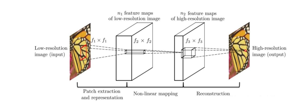
该网络对于一个低分辨率图像,先使用双三次插值将其放大到目标大小,再通过三层卷积网络做非线性映射,得到的结果作为高分辨率图像输出。
作者对于这三层卷积层的解释:
(1)特征块提取和表示:此操作从低分辨率图像Y中提取重叠特征块,并将每个特征块表示为一个高维向量。这些向量包括一组特征图,其数量等于向量的维数。
(2)非线性映射:该操作将每个高维向量非线性映射到另一个高维向量。每个映射向量在概念上都是高分辨率特征块的表示。这些向量同样包括另一组特征图。
(3)重建:该操作聚合上述高分辨率patch-wise(介于像素级别和图像级别的区域)表示,生成最终的高分辨率图像。
各层结构:
- 输入:处理后的低分辨率图像
- 卷积层 1:采用 9×9 的卷积核
- 卷积层 2:采用 1×1 的卷积核
- 卷积层 3:采用 5×5 的卷积核
- 输出:高分辨率图像
模型结构代码:
class SRCNN(nn.Module):
    def __init__(self, upscale_factor):
        super(SRCNN, self).__init__()

        self.relu = nn.ReLU()
        self.conv1 = nn.Conv2d(1, 64, kernel_size=5, stride=1, padding=2)
        self.conv2 = nn.Conv2d(64, 64, kernel_size=3, stride=1, padding=1)
        self.conv3 = nn.Conv2d(64, 32, kernel_size=3, stride=1, padding=1)
        self.conv4 = nn.Conv2d(32, upscale_factor ** 2,
                               kernel_size=3, stride=1, padding=1)
        self.pixel_shuffle = nn.PixelShuffle(upscale_factor)

        self._initialize_weights()

    def _initialize_weights(self):
        init.orthogonal_(self.conv1.weight, init.calculate_gain('relu'))
        init.orthogonal_(self.conv2.weight, init.calculate_gain('relu'))
        init.orthogonal_(self.conv3.weight, init.calculate_gain('relu'))
        init.orthogonal_(self.conv4.weight)

    def forward(self, x):
        x = self.conv1(x)
        x = self.relu(x)
        x = self.conv2(x)
        x = self.relu(x)
        x = self.conv3(x)
        x = self.relu(x)
        x = self.conv4(x)
        x = self.pixel_shuffle(x)
        return x
4.2 FSRCNN
FSRCNN 由 2016 年 Chao Dong 等人提出,与 SRCNN 是相同作者。其网络结构如下图所示: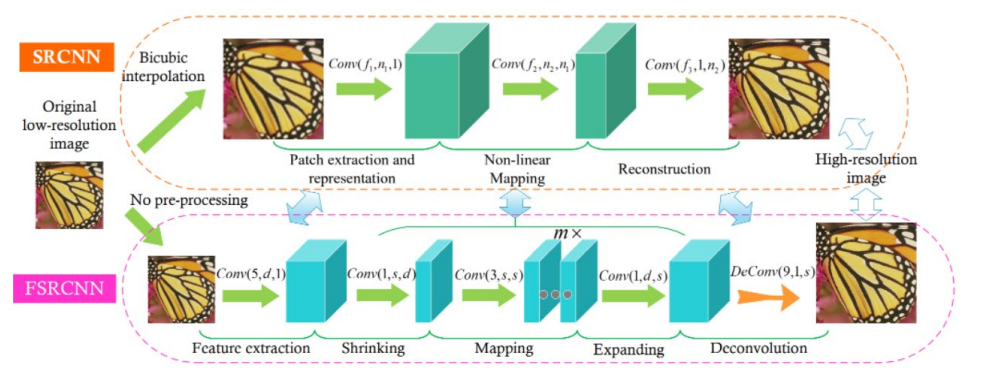
FSRCNN在SRCNN基础上做了如下改变:
1.FSRCNN直接采用低分辨的图像作为输入,不同于SRCNN需要先对低分辨率的图像进行双三次插值然后作为输入;
2.FSRCNN在网络的最后采用反卷积层实现上采样;
3.FSRCNN中没有非线性映射,相应地出现了收缩、映射和扩展;
4.FSRCNN选择更小尺寸的滤波器和更深的网络结构。
各层结构:
- 输入层:FSRCNN不使用bicubic插值来对输入图像做上采样,它直接进入特征提取层
- 特征提取层:采用1 × d × ( 5 × 5 )的卷积层提取
- 收缩层:采用d × s × ( 1 × 1 ) 的卷积层去减少通道数,来减少模型复杂度
- 映射层:采用s × s × ( 3 × 3 ) 卷积层去增加模型非线性度来实现LR → SR 的映射
- 扩张层:该层和收缩层是对称的,采用s × d × ( 1 × 1 ) 卷积层去增加重建的表现力
- 反卷积层:s × 1 × ( 9 × 9 )
- 输出层:输出HR图像
模型结构代码:
class FSRCNN(nn.Module):
    def __init__(self, scale_factor, num_channels=1, d=56, s=12, m=4):
        super(FSRCNN, self).__init__()
        self.first_part = nn.Sequential(
            nn.Conv2d(num_channels, d, kernel_size=5, padding=5//2),
            nn.PReLU(d)
        )
        self.mid_part = [nn.Conv2d(d, s, kernel_size=1), nn.PReLU(s)]
        for _ in range(m):
            self.mid_part.extend([nn.Conv2d(s, s, kernel_size=3, padding=3//2), nn.PReLU(s)])
        self.mid_part.extend([nn.Conv2d(s, d, kernel_size=1), nn.PReLU(d)])
        self.mid_part = nn.Sequential(*self.mid_part)
        self.last_part = nn.ConvTranspose2d(d, num_channels, kernel_size=9, stride=scale_factor, padding=9//2,
                                            output_padding=scale_factor-1)

        self._initialize_weights()

    def _initialize_weights(self):
        for m in self.first_part:
            if isinstance(m, nn.Conv2d):
                nn.init.normal_(m.weight.data, mean=0.0, std=math.sqrt(2/(m.out_channels*m.weight.data[0][0].numel())))
                nn.init.zeros_(m.bias.data)
        for m in self.mid_part:
            if isinstance(m, nn.Conv2d):
                nn.init.normal_(m.weight.data, mean=0.0, std=math.sqrt(2/(m.out_channels*m.weight.data[0][0].numel())))
                nn.init.zeros_(m.bias.data)
        nn.init.normal_(self.last_part.weight.data, mean=0.0, std=0.001)
        nn.init.zeros_(self.last_part.bias.data)

    def forward(self, x):
        x = self.first_part(x)
        x = self.mid_part(x)
        x = self.last_part(x)
        return x
5.评估指标
本次实验尝试了 PSNR 和 SSIM 两个指标。
5.1 PSNR
PSNR(Peak Signal to Noise Ratio)为峰值信噪比,计算公式如下: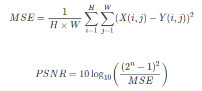
其中,n为每像素的比特数。
PSNR 的单位是dB,数值越大表示失真越小,一般认为 PSNR 在 38 以上的时候,人眼就无法区分两幅图片了。
相关代码:
def psnr(loss):
    return 10 * log10(1 / loss.item())
5.2 SSIM
SSIM(Structural Similarity)为结构相似性,由三个对比模块组成:亮度、对比度、结构。
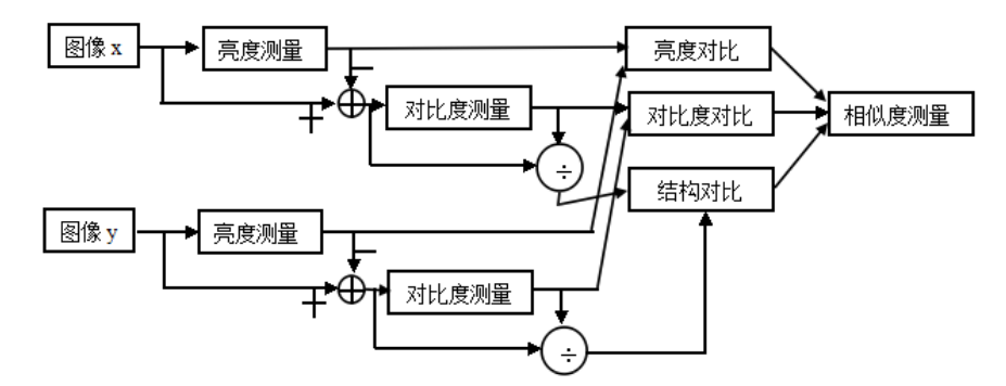
亮度对比函数
图像的平均灰度计算公式: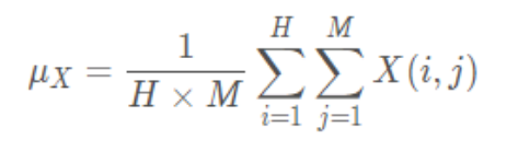
亮度对比函数计算公式: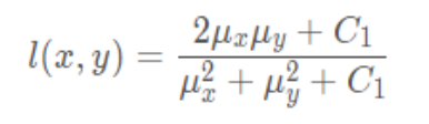
对比度对比函数
图像的标准差计算公式: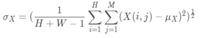
对比度对比函数计算公式: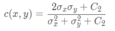
结构对比函数
结构对比函数计算公式: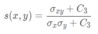
综合上述三个部分,得到 SSIM 计算公式: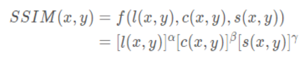
其中, α \alpha α, β \beta β, γ \gamma γ > 0,用来调整这三个模块的重要性。
SSIM 函数的值域为[0, 1], 值越大说明图像失真越小,两幅图像越相似。
相关代码:
由于pytorch没有类似tensorflow类似tf.image.ssim这样计算SSIM的接口,因此根据公式进行自定义函数用来计算
""" 计算ssim函数 """
# 计算一维的高斯分布向量
def gaussian(window_size, sigma):
    gauss = torch.Tensor(
        [exp(-(x - window_size//2)**2/float(2*sigma**2)) for x in range(window_size)])
    return gauss/gauss.sum()


# 创建高斯核,通过两个一维高斯分布向量进行矩阵乘法得到
# 可以设定channel参数拓展为3通道
def create_window(window_size, channel=1):
    _1D_window = gaussian(window_size, 1.5).unsqueeze(1)
    _2D_window = _1D_window.mm(
        _1D_window.t()).float().unsqueeze(0).unsqueeze(0)
    window = _2D_window.expand(
        channel, 1, window_size, window_size).contiguous()
    return window


# 计算SSIM
# 直接使用SSIM的公式,但是在计算均值时,不是直接求像素平均值,而是采用归一化的高斯核卷积来代替。
# 在计算方差和协方差时用到了公式Var(X)=E[X^2]-E[X]^2, cov(X,Y)=E[XY]-E[X]E[Y].
def ssim(img1, img2, window_size=11, window=None, size_average=True, full=False, val_range=None):
    # Value range can be different from 255. Other common ranges are 1 (sigmoid) and 2 (tanh).
    if val_range is None:
        if torch.max(img1) > 128:
            max_val = 255
        else:
            max_val = 1

        if torch.min(img1) < -0.5:
            min_val = -1
        else:
            min_val = 0
        L = max_val - min_val
    else:
        L = val_range

    padd = 0
    (_, channel, height, width) = img1.size()
    if window is None:
        real_size = min(window_size, height, width)
        window = create_window(real_size, channel=channel).to(img1.device)

    mu1 = F.conv2d(img1, window, padding=padd, groups=channel)
    mu2 = F.conv2d(img2, window, padding=padd, groups=channel)

    mu1_sq = mu1.pow(2)
    mu2_sq = mu2.pow(2)
    mu1_mu2 = mu1 * mu2

    sigma1_sq = F.conv2d(img1 * img1, window, padding=padd,
                         groups=channel) - mu1_sq
    sigma2_sq = F.conv2d(img2 * img2, window, padding=padd,
                         groups=channel) - mu2_sq
    sigma12 = F.conv2d(img1 * img2, window, padding=padd,
                       groups=channel) - mu1_mu2

    C1 = (0.01 * L) ** 2
    C2 = (0.03 * L) ** 2

    v1 = 2.0 * sigma12 + C2
    v2 = sigma1_sq + sigma2_sq + C2
    cs = torch.mean(v1 / v2)  # contrast sensitivity

    ssim_map = ((2 * mu1_mu2 + C1) * v1) / ((mu1_sq + mu2_sq + C1) * v2)

    if size_average:
        ret = ssim_map.mean()
    else:
        ret = ssim_map.mean(1).mean(1).mean(1)

    if full:
        return ret, cs
    return ret


class SSIM(torch.nn.Module):
    def __init__(self, window_size=11, size_average=True, val_range=None):
        super(SSIM, self).__init__()
        self.window_size = window_size
        self.size_average = size_average
        self.val_range = val_range

        # Assume 1 channel for SSIM
        self.channel = 1
        self.window = create_window(window_size)

    def forward(self, img1, img2):
        (_, channel, _, _) = img1.size()

        if channel == self.channel and self.window.dtype == img1.dtype:
            window = self.window
        else:
            window = create_window(self.window_size, channel).to(
                img1.device).type(img1.dtype)
            self.window = window
            self.channel = channel

        return ssim(img1, img2, window=window, window_size=self.window_size, size_average=self.size_average)
6.模型训练/测试
设定 epoch 为 500 次,保存验证集上 PSNR 最高的模型。两个模型在测试集上的表现如下表所示: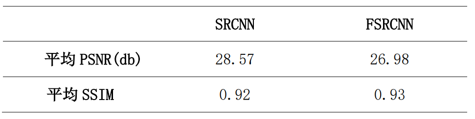
从结果可以发现,FSRCNN 的 PSNR 比 SRCNN 低,但 FSRCNN 的 SSIM 比 SRCNN 高,说明 PSNR 和 SSIM 并不存在完全正相关的关系。
训练/验证代码:
model = FSRCNN(1).to(device)
criterion = nn.MSELoss()
optimizer = optim.Adam(model.parameters(), lr=1e-2)
scheduler = MultiStepLR(optimizer, milestones=[50, 75, 100], gamma=0.1)
best_psnr = 0.0
for epoch in range(nb_epochs):
    # Train
    epoch_loss = 0
    for iteration, batch in enumerate(trainloader):
        input, target = batch[0].to(device), batch[1].to(device)
        optimizer.zero_grad()
        out = model(input)
        loss = criterion(out, target)
        loss.backward()
        optimizer.step()
        epoch_loss += loss.item()
    print(f"Epoch {
      epoch}. Training loss: {
      epoch_loss / len(trainloader)}")
    # Val
    sum_psnr = 0.0
    sum_ssim = 0.0
    with torch.no_grad():
        for batch in valloader:
            input, target = batch[0].to(device), batch[1].to(device)
            out = model(input)
            loss = criterion(out, target)
            pr = psnr(loss)
            sm = ssim(input, out)
            sum_psnr += pr
            sum_ssim += sm
    print(f"Average PSNR: {
      sum_psnr / len(valloader)} dB.")
    print(f"Average SSIM: {
      sum_ssim / len(valloader)} ")
    avg_psnr = sum_psnr / len(valloader)
    if avg_psnr >= best_psnr:
        best_psnr = avg_psnr
        torch.save(model, r"best_model_FSRCNN.pth")
    scheduler.step()
测试代码:
BATCH_SIZE = 4
model_path = "best_model_FSRCNN.pth"
testset = DatasetFromFolder(r"./data/images/test", zoom_factor)
testloader = DataLoader(dataset=testset, batch_size=BATCH_SIZE,
                        shuffle=False, num_workers=NUM_WORKERS)
sum_psnr = 0.0
sum_ssim = 0.0
model = torch.load(model_path).to(device)
criterion = nn.MSELoss()
with torch.no_grad():
    for batch in testloader:
        input, target = batch[0].to(device), batch[1].to(device)
        out = model(input)
        loss = criterion(out, target)
        pr = psnr(loss)
        sm = ssim(input, out)
        sum_psnr += pr
        sum_ssim += sm
print(f"Test Average PSNR: {
      sum_psnr / len(testloader)} dB")
print(f"Test Average SSIM: {
      sum_ssim / len(testloader)} ")
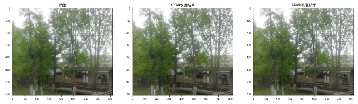
7.实图测试
为了直观感受两个模型的效果,我用自己拍摄的图进行实图测试,效果如下:
s=1(放大倍数=1)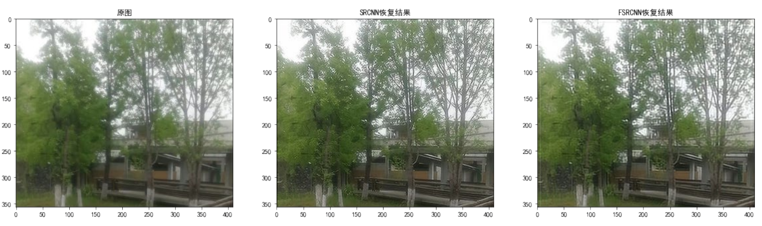
当放大倍数=1时,SRCNN的超分结果比FSRCNN的超分效果要更好一些,这和两个模型平均 PSNR 的数值相吻合。
s=2(放大倍数=2)
当放大倍数=2时,SRCNN 的超分结果和 FSRCNN 的超分效果相差不大。
相关代码:
# 参数设置
zoom_factor = 1
model = "best_model_SRCNN.pth"
model2 = "best_model_FSRCNN.pth"
image = "tree.png"
cuda = 'store_true'
device = torch.device("cuda:0" if torch.cuda.is_available() else "cpu")

# 读取图片
img = Image.open(image).convert('YCbCr')
img = img.resize((int(img.size[0] * zoom_factor), int(img.size[1] * zoom_factor)), Image.BICUBIC)
y, cb, cr = img.split()
img_to_tensor = transforms.ToTensor()
input = img_to_tensor(y).view(1, -1, y.size[1], y.size[0]).to(device)

# 输出图片
model = torch.load(model).to(device)
out = model(input).cpu()
out_img_y = out[0].detach().numpy()
out_img_y *= 255.0
out_img_y = out_img_y.clip(0, 255)
out_img_y = Image.fromarray(np.uint8(out_img_y[0]), mode='L')
out_img = Image.merge('YCbCr', [out_img_y, cb, cr]).convert('RGB')

model2 = torch.load(model2).to(device)
out2 = model2(input).cpu()
out_img_y2 = out2[0].detach().numpy()
out_img_y2 *= 255.0
out_img_y2 = out_img_y2.clip(0, 255)
out_img_y2 = Image.fromarray(np.uint8(out_img_y2[0]), mode='L')
out_img2 = Image.merge('YCbCr', [out_img_y2, cb, cr]).convert('RGB')

# 绘图显示
fig, ax = plt.subplots(1, 3, figsize=(20, 20))
ax[0].imshow(img)
ax[0].set_title("原图")
ax[1].imshow(out_img)
ax[1].set_title("SRCNN恢复结果")
ax[2].imshow(out_img2)
ax[2].set_title("FSRCNN恢复结果")
plt.show()
fig.savefig(r"tree2.png")
源码获取
实验报告,完整的源码文件,数据集获取:
https://download.csdn.net/download/qq1198768105/85906814
边栏推荐
- Compile advanced notes
- Win10 or win11 taskbar, automatically hidden and transparent
- Novel Slot Detection: A Benchmark for Discovering Unknown Slot Types in the Dialogue System
- Ctfshow, information collection: web9
- PG基础篇--逻辑结构管理(锁机制--表锁)
- Shengteng experience officer Episode 5 notes I
- Ctfshow, information collection: web6
- Webrtc audio anti weak network technology (Part 1)
- 防火墙基础之服务器区的防护策略
- Niuke real problem programming - Day12
猜你喜欢
Ctfshow, information collection: web9
C 6.0 language specification approved

Ctfshow, information collection: web10
Full details of efficientnet model
Ctfshow, information collection: web5
Ctfshow, information collection: web6

Stm32cubemx, 68 sets of components, following 10 open source protocols

The world's first risc-v notebook computer is on pre-sale, which is designed for the meta universe!

CTFshow,信息搜集:web14

Promoted to P8 successfully in the first half of the year, and bought a villa!
随机推荐
Read PG in data warehouse in one article_ stat
[机缘参悟-40]:方向、规则、选择、努力、公平、认知、能力、行动,读3GPP 6G白皮书的五层感悟
FFmpeg----图片处理
@Introduction and three usages of controlleradvice
Ctfshow, information collection: web2
Yyds dry goods inventory # solve the real problem of famous enterprises: cross line
Infinite innovation in cloud "vision" | the 2022 Alibaba cloud live summit was officially launched
Today's sleep quality record 78 points
CTFshow,信息搜集:web5
一文读懂数仓中的pg_stat
Attribute keywords serveronly, sqlcolumnnumber, sqlcomputecode, sqlcomputed
Compile advanced notes
数据库如何进行动态自定义排序?
Wechat applet - Advanced chapter component packaging - Implementation of icon component (I)
Delete a whole page in word
Attribute keywords ondelete, private, readonly, required
Lidar Knowledge Drop
Novel Slot Detection: A Benchmark for Discovering Unknown Slot Types in the Dialogue System
上半年晋升 P8 成功,还买了别墅!
Apache多个组件漏洞公开(CVE-2022-32533/CVE-2022-33980/CVE-2021-37839)