当前位置:网站首页>Mathematical modeling for war preparation 33- grey prediction model 2
Mathematical modeling for war preparation 33- grey prediction model 2
2022-06-30 16:40:00 【nuist__ NJUPT】
Catalog
Two 、3 Kind of GM(1,1) Basic principle and implementation steps of the model
This section mainly studies the concept and basic principle of grey system , And three kinds of grey prediction models are introduced , The specific steps of grey prediction are given , At the same time, three kinds of grey prediction are compared and analyzed , A classic case of grey prediction is given , And gives MATLAB Code and case analysis , Finally, the applicable scope of the prediction model and the grey prediction model is summarized and analyzed , Now let's start to study hard !
One 、 Concept of grey system
Let's look at the concept of grey system , That is, some data of the system is known , Part of the data is unknown , It is called grey system , The grey prediction is to generate regular data sequence by accumulating the original data sequence in turn , Then the corresponding differential equation is established , So as to predict the development trend of future things .

GM(1,1) The model is suitable for Primitive discrete nonnegative sequence , It is better to use the year as the abscissa and the data is greater than or equal to 4 period , Generally, we only consider one accumulation of one variable .

Two 、3 Kind of GM(1,1) Basic principle and implementation steps of the model
It is necessary to test the quasi exponential law of the data before grey prediction , There are also books that say that the level comparison test should be carried out , Only after passing the inspection can we consider using Grey prediction , otherwise , Grey prediction cannot be used .

After passing the quasi exponential law test and the order ratio test , We draw a time series diagram of the original data to observe whether it is a non negative sequence , And then, an accumulation sum is performed to find the nearest mean value to generate a sequence .

Next, we construct a grey prediction model , The least square method is used to estimate the parameters , Get the parameters a and b.

Last , Let's talk about the transformation of grey equation into non whitened equation , And solve , Then, the sequence can be restored to the original sequence before accumulation forecast .

Of course , It is also necessary to test the residual error and grade deviation of the model , Only through the test can it be shown that the prediction deviation of Mo model is small , It can meet the forecast demand , Otherwise, the prediction effect of the grey prediction model is poor .


We can use three GM contrast , Divide the data into training group and test group , Judge which model has good prediction effect , Which one to use , Or take the mean value of the three sum models directly . Tradition GM Is to use the old data to predict , The new information is to add the forecast information every time and then make the forecast , Metabolism is to eliminate old information and then add information to predict each time .

3、 ... and 、 Classic case
Let's take a look at this example , For giving the past of the Yangtze River 10 Pollution in , Predicting the future 10 Pollution in .
The process of analyzing the above topics is as follows , First, draw the time series diagram of the original data , It is obvious that the number of periods measured by year is greater than 4 The data of , So we can consider the grey prediction model , Then there is the quasi exponential law test and the order ratio test , Pass the test , Grey prediction model can be used , Then because of 10 period , front 8 Divided into training groups , The last two phases are the experimental group , Select the sum of squares of errors SSE The smallest grey prediction model is used for prediction , Finally, the time sequence diagram of the predicted data and the original data is drawn and the results are displayed , At the same time, residual error test and order ratio deviation test are required .


MATLAB The main function code is as follows :
clear; clc
year = 1995:1:2004; % year
x0 = [174,179,183,189,207,234,220.5,256,270,285] ;% Raw data sequence
n = length(x0);
year = year' ;
x0 = x0' ;

% Draw a sequence diagram , Observe whether it is non negative data measured by year
figure(1) ;
plot(year, x0, 'o-') ;
grid on ;
set(gca,'xtick',year(1:1:end)) ; % Set up x The spacing of the shafts is 1
xlabel(' year ');  ylabel(' Total sewage discharge ');

%GM The model is suitable for non negative sequences with short data , So a nonnegative test is required
ERROR = 0;  %  Establish an error indicator , Once there is an error, it is specified as 1
%  Determine whether there are negative elements , Of course, the amount of data should be 4~10 It is only after a period of time that GM
if sum(x0<0) > 0
    disp(' The original data has a negative value , Out of commission GM')
    ERROR = 1;
end

% Carry out the quasi exponential law test and the order ratio test
if ERROR == 0
    disp('------------------------------------------------------------')
    disp(' Quasi exponential law test ')
    x1 = cumsum(x0);   %  One time accumulation
    rho = x0(2:end) ./ x1(1:end-1) ;   %  Calculate smoothness rho(k) = x0(k)/x1(k-1)

    %  Draw a graph of smoothness , And draw 0.5 The straight line of , It means the critical value
    figure(2)
    plot(year(2:end),rho,'o-',[year(2),year(end)],[0.5,0.5],'-'); grid on;
    text(year(end-1)+0.2,0.55,' The critical line ')   %  In coordinates (year(end-1)+0.2,0.55) Add text to
    set(gca,'xtick',year(2:1:end))  %  Set up x The interval between the axis abscissa is 1
    xlabel(' year ');  ylabel(' Smoothness of raw data ');  %  Label the axis


    disp(strcat(' indicators 1: The smoothness ratio is less than 0.5 The proportion of data is ',num2str(100*sum(rho<0.5)/(n-1)),'%'))
    disp(strcat(' indicators 2: Except for the first two periods , The smoothness ratio is less than 0.5 The proportion of data is ',num2str(100*sum(rho(3:end)<0.5)/(n-3)),'%'))
    disp(' Reference standards : indicators 1 Generally greater than 60%,  indicators 2 Be greater than 90%, Do you think the data of this example can pass the test ?')

    flag = 1 ;
    for k = 2 : n
    lamda(k) = x0(k-1) / x0(k) ;
    if (lamda(k) < exp(-2 / (n+1)) || lamda(k) > exp(2 / (n+1)))
        disp(' Fail the grade ratio test !!!') ;
        flag = 0 ;
    end
    end
    if flag == 1
        disp(' Pass the grade ratio test !!!') ;
    end
       % Draw the level ratio test chart
    figure(3)
    x3 = 1: length(lamda)-1 ;
    plot(x3, lamda(2:end), 'o-',[x3(1),x3(end)],[exp(2 / (n+1)),exp(2 / (n+1))],[x3(1),x3(end)],[exp(-2 / (n+1)),exp(-2 / (n+1))]) ;
    grid on ;
    text(2,exp(2 / (n+1)+0.05),' Upper limit of stage ratio ') ;
    text(2,exp(-2 / (n+1)-0.05),' Lower limit of stage ratio ') ;
    set(gca,'xtick',x3(1:1:end)) ;
    set(gca,'ytick',0.5:0.1:1.5) ;
    axis([1 x3(end) 0.5 1.5]) ;
    xlabel(' Number of stage ratios ');  ylabel(' Grade ratio ');

    Judge = input(' Do you think it can pass the test of quasi exponential law ? Yes, please enter 1, No, please enter 0:');
    if Judge == 0
        disp(' Pro - , The grey prediction model is not suitable for your data ~  Please consider other methods   for example ARIMA, Exponential smoothing, etc ')
        ERROR = 1;
    end

    disp('------------------------------------------------------------')
end

%%  When the amount of data is greater than 4 when , We used the experimental group to choose to use the traditional GM(1,1) Model 、 New information GM(1,1) Model or metabolism GM(1,1) Model ;  If the amount of data is equal to 4, Then we directly calculate an average of the three methods to predict
if ERROR == 0 && flag == 1  %  If none of the above errors occur , To perform the following steps
    if  n > 4  %  The amount of data is greater than 4 when , The data were divided into training group and experimental group ( According to the original data size n Come and get it ,n by 5-7 The last two years were taken as the experimental group ,n Greater than 7 Take the last three years as the experimental group )
        disp(' Because the number of periods of the original data is greater than 4, So we can divide the data into training group and experimental group ')   %  Be careful , If the number of test groups is only 1 individual , Then the results of the three models are exactly the same , So at least take 2 A test group
        if n > 7
            test_num = 3;
        else
            test_num = 2;
        end
        train_x0 = x0(1:end-test_num);  %  Training data
        disp(' The training data is : ')
        disp(mat2str(train_x0'))  % mat2str You can convert a matrix or vector into a string display ,  Adding a prime here means transpose , Turn the column vector into a row vector for easy viewing
        test_x0 =  x0(end-test_num+1:end); %  Test data
        disp(' The test data are : ')
        disp(mat2str(test_x0'))  % mat2str You can convert a matrix or vector into a string display
        disp('------------------------------------------------------------')

        %  Three models are used to train the training data , Back to result Is to predict later test_num Data for the period
        disp(' ')
        disp('*** Here is the traditional GM(1,1) The detailed process of model prediction ***')
        result1 = gm11(train_x0, test_num); % Use traditional GM(1,1) The model is applied to the training data , And predict test_num The results of the period
        disp(' ')
        disp('*** Here's how to make new information GM(1,1) The detailed process of model prediction ***')
        result2 = new_gm11(train_x0, test_num); % Use new information GM(1,1) The model is applied to the training data , And predict test_num The results of the period
        disp(' ')
        disp('*** Here's how to metabolize GM(1,1) The detailed process of model prediction ***')
        result3 = metabolism_gm11(train_x0, test_num); % Use metabolism GM(1,1) The model is applied to the training data , And predict test_num The results of the period

        %  Now compare the prediction results of the three models for the experimental data
        disp(' ')
        disp('------------------------------------------------------------')
        %  Draw a graph to predict the test data ( For some data , Maybe the results predicted by the three straight lines are very close )
        test_year = year(end-test_num+1:end);  %  The year corresponding to the test group
        figure(4);
        plot(test_year,test_x0,'o-',test_year,result1,'*-',test_year,result2,'+-',test_year,result3,'x-'); grid on;
        set(gca,'xtick',year(end-test_num+1): 1 :year(end))  %  Set up x The interval between the axis abscissa is 1
        legend(' The real data of the test group ',' Tradition GM(1,1) Predicted results ',' New information GM(1,1) Predicted results ',' The new supersedes the old GM(1,1) Predicted results ')  %  Be careful : If lengend Blocking the line in the figure , that lengend You can manually drag the position of
        xlabel(' year ');  ylabel(' Total sewage discharge ');  %  Label the axis
        %  Calculate the sum of squares of errors SSE
        SSE1 = sum((test_x0-result1).^2);
        SSE2 = sum((test_x0-result2).^2);
        SSE3 = sum((test_x0-result3).^2);
        disp(strcat(' Tradition GM(1,1) For the experimental group, the sum of squares of the predicted errors is ',num2str(SSE1)))
        disp(strcat(' New information GM(1,1) For the experimental group, the sum of squares of the predicted errors is ',num2str(SSE2)))
        disp(strcat(' The new supersedes the old GM(1,1) For the experimental group, the sum of squares of the predicted errors is ',num2str(SSE3)))
        if SSE1<SSE2
            if SSE1<SSE3
                choose = 1;  % SSE1 Minimum , Choose tradition GM(1,1) Model
            else
                choose = 3;  % SSE3 Minimum , Choose metabolism GM(1,1) Model
            end
        elseif SSE2<SSE3
            choose = 2;  % SSE2 Minimum , Select new information GM(1,1) Model
        else
            choose = 3;  % SSE3 Minimum , Choose metabolism GM(1,1) Model
        end
        Model = {' Tradition GM(1,1) Model ',' New information GM(1,1) Model ',' The new supersedes the old GM(1,1) Model '};
        disp(strcat(' because ',Model(choose),' The sum of squares of errors is the smallest , So we should choose it for prediction '))
        disp('------------------------------------------------------------')

%  Choose the model with the least error to predict
        predict_num = input(' Please enter the number of periods you want to forecast later : ');
        %  The calculation uses traditional GM The result of the model , To get another return variable :x0_hat,  Relative residuals relative_residuals And order ratio deviation eta
        [result, x0_hat, relative_residuals, eta] = gm11(x0, predict_num);  %  First use of gm11 Function to get the detailed results of fitting the original data

        % %  Judge which model we choose , If it is 2 or 3, Then the update was just made by the model 1 The calculated prediction results
        if choose == 2
            result = new_gm11(x0, predict_num);
        end
        if choose == 3
            result = metabolism_gm11(x0, predict_num);
        end
%  Output the results predicted by the best model
        disp('------------------------------------------------------------')
        disp(' The fitting results of the original data :')
        for i = 1:n
            disp(strcat(num2str(year(i)), ' : ',num2str(x0_hat(i))))
        end
        disp(strcat(' Predict later ',num2str(predict_num),' The results of the period :'))
        for i = 1:predict_num
            disp(strcat(num2str(year(end)+i), ' : ',num2str(result(i))))
        end
     %  If there are only four periods of data , Then we don't have to choose which model to predict , Directly calculate an average of the predicted results of the three models ~
    else
        disp(' Because the data is just 4 period , Therefore, we can directly average the results of the three methods ~')
        predict_num = input(' Please enter the number of periods you want to forecast later : ');
        disp(' ')
        disp('*** Here is the traditional GM(1,1) The detailed process of model prediction ***')
        [result1, x0_hat, relative_residuals, eta] = gm11(x0, predict_num);
        disp(' ')
        disp('*** Here's how to make new information GM(1,1) The detailed process of model prediction ***')
        result2 = new_gm11(x0, predict_num);
        disp(' ')
        disp('*** Here's how to metabolize GM(1,1) The detailed process of model prediction ***')
        result3 = metabolism_gm11(x0, predict_num);
        result = (result1+result2+result3)/3;

        disp(' The fitting results of the original data :')
        for i = 1:n
            disp(strcat(num2str(year(i)), ' : ',num2str(x0_hat(i))))
        end
        disp(strcat(' Tradition GM(1,1) Predict later ',num2str(predict_num),' The results of the period :'))
        for i = 1:predict_num
            disp(strcat(num2str(year(end)+i), ' : ',num2str(result1(i))))
        end
        disp(strcat(' New information GM(1,1) Predict later ',num2str(predict_num),' The results of the period :'))
        for i = 1:predict_num
            disp(strcat(num2str(year(end)+i), ' : ',num2str(result2(i))))
        end
        disp(strcat(' The new supersedes the old GM(1,1) Predict later ',num2str(predict_num),' The results of the period :'))
        for i = 1:predict_num
            disp(strcat(num2str(year(end)+i), ' : ',num2str(result3(i))))
        end
        disp(strcat(' The future prediction obtained by averaging the three methods ',num2str(predict_num),' The results of the period :'))
        for i = 1:predict_num
            disp(strcat(num2str(year(end)+i), ' : ',num2str(result(i))))
        end
    end
      %  Draw a graph of relative residual and order ratio deviation ( Be careful : Because it is the evaluation of the fitting effect of the original data , So the three models are the same ~~~)
    figure(5)
    subplot(2,1,1)  %  Draw a subgraph ( Block the diagram )
    plot(year(2:end), relative_residuals,'*-'); grid on;   %  Each period and relative residual in the original data
    legend(' Relative residuals '); xlabel(' year ');
    set(gca,'xtick',year(2:1:end))  %  Set up x The interval between the axis abscissa is 1
    subplot(2,1,2)
    plot(year(2:end), eta,'o-'); grid on;   %  Deviation of each period and grade ratio in the original data
    legend(' Order ratio deviation '); xlabel(' year ');
    set(gca,'xtick',year(2:1:end))  %  Set up x The interval between the axis abscissa is 1
    disp(' ')
    disp('**** Next, the evaluation results of the original data fitting will be output ***')

    %%  Residual test
    average_relative_residuals = mean(relative_residuals);  %  Calculate the average relative residual  mean The function is used to mean
    disp(strcat(' The average relative residual is ',num2str(average_relative_residuals)))
    if average_relative_residuals<0.1
        disp(' The results of residual test show that : The fitting degree of the model to the original data is very good ')
    elseif average_relative_residuals<0.2
        disp(' The results of residual test show that : The fitting degree of the model to the original data meets the general requirements ')
    else
        disp(' The results of residual test show that : The fitting degree of the model to the original data is not very good , It is recommended to use other models to predict ')
    end

    %  Level ratio deviation inspection
    average_eta = mean(eta);   %  Calculate the average order ratio deviation
    disp(strcat(' The average order ratio deviation is ',num2str(average_eta)))
    if average_eta<0.1
        disp(' The results of order ratio deviation test show that : The fitting degree of the model to the original data is very good ')
    elseif average_eta<0.2
        disp(' The results of order ratio deviation test show that : The fitting degree of the model to the original data meets the general requirements ')
    else
        disp(' The results of order ratio deviation test show that : The fitting degree of the model to the original data is not very good , It is recommended to use other models to predict ')
    end
    disp(' ')
    disp('------------------------------------------------------------')

    %  Draw the final prediction effect diagram
    figure(6)  %  The symbols in the drawing below m: Magenta  b: Blue
    plot(year,x0,'-o',  year,x0_hat,'-*m',  year(end)+1:year(end)+predict_num,result,'-*b' );   grid on;
    hold on;
    plot([year(end),year(end)+1],[x0(end),result(1)],'-*b')
    legend(' Raw data ',' Fitting data ',' Forecast data ')  %  Be careful : If lengend Blocking the line in the figure , that lengend You can manually drag the position of
    set(gca,'xtick',[year(1):1:year(end)+predict_num])  %  Set up x The interval between the axis abscissa is 1
    xlabel(' year ');  ylabel(' Total sewage discharge ');  %  Label the axis
end
Tradition GM(1,1) The model function code is as follows :
function [result, x0_hat, relative_residuals, eta] = gm11(x0, predict_num)
    %  Function function : Use traditional GM(1,1) The model predicts the data
    %     x0: Raw data to be predicted
    %     predict_num:  Number of backward forecast periods
    %  Output variables  ( Be careful , When the function is actually called, it does not necessarily output all the results , It's like corrcoef The function is the same ~, You can only output the correlation coefficient matrix , You can also attach output p Value matrix )
    %     result: Predictive value
    %     x0_hat: The fitting value of the original data
    %     relative_residuals:  The relative residual calculated when evaluating the model
    %     eta:  The order ratio deviation calculated when evaluating the model

    n = length(x0); %  Length of data
    x1=cumsum(x0); %  Calculate the cumulative value once
    z1 = (x1(1:end-1) + x1(2:end)) / 2;  %  Calculate the nearest mean to generate a sequence ( The length is n-1)
    %  Will start with the second item x0 As a y,z1 As a x, To make a unitary regression   y = kx +b
    y = x0(2:end); x = z1;
    %  The following expression is the expression in the Fourth Lecture fitting ~  But be careful , The number of samples should be n-1, One item is missing
    k = ((n-1)*sum(x.*y)-sum(x)*sum(y))/((n-1)*sum(x.*x)-sum(x)*sum(x));
    b = (sum(x.*x)*sum(y)-sum(x)*sum(x.*y))/((n-1)*sum(x.*x)-sum(x)*sum(x));
    a = -k;  % Be careful :k = -a Oh
    %  Be careful : -a Is the development coefficient ,  b Is the amount of ash

    disp(' For now GM(1,1) The raw data of the forecast is : ')
    disp(mat2str(x0'))  % mat2str You can convert a matrix or vector into a string display
    disp(strcat(' The development coefficient fitted by the least square method is ',num2str(-a),', The amount of ash action is ',num2str(b)))
    disp('*************** Split line ***************')
    x0_hat=zeros(n,1);  x0_hat(1)=x0(1);   % x0_hat Vectors are used to store pairs of x0 The fitting value of the sequence , Here is the initialization
    for m = 1: n-1
        x0_hat(m+1) = (1-exp(a))*(x0(1)-b/a)*exp(-a*m);
    end
    result = zeros(predict_num,1);  %  Initialize the vector used to save the predicted value
    for i = 1: predict_num
        result(i) = (1-exp(a))*(x0(1)-b/a)*exp(-a*(n+i-1)); %  Bring in the formula and calculate directly
    end

    %  Calculate the absolute and relative residuals
    absolute_residuals = x0(2:end) - x0_hat(2:end);   %  Calculate the absolute residual from the second term , Because the first item is the same
    relative_residuals = abs(absolute_residuals) ./ x0(2:end);  %  Calculate the relative residual , Pay attention to the absolute value of the molecule , And use dot division
    %  Calculate the stage ratio and the stage ratio deviation
    class_ratio = x0(2:end) ./ x0(1:end-1) ;  %  Calculate the stage ratio  sigma(k) = x0(k)/x0(k-1)
    eta = abs(1-(1-0.5*a)/(1+0.5*a)*(1./class_ratio));  %  Calculate the stage ratio deviation
end
New information GM(1,1) Model function code :
function [result] = new_gm11(x0, predict_num)
%  Function function : Using new information GM(1,1) The model predicts the data
%  The input variable
%     x0: Raw data to be predicted
%     predict_num:  Number of backward forecast periods
%  Output variables
%     result: Predictive value
    result = zeros(predict_num,1);  %  Initialize the vector used to save the predicted value
    for i = 1 : predict_num
        result(i) = gm11(x0, 1);  %  Save the results of phase I forecast to result in
        x0 = [x0; result(i)];  %  to update x0 vector , here x0 With new prediction information
    end
end
The new supersedes the old GM(1,1) Model function code :
function [result] = metabolism_gm11(x0, predict_num)
%  Function function : Use metabolic GM(1,1) The model predicts the data
%  The input variable
%     x0: Raw data to be predicted
%     predict_num:  Number of backward forecast periods
%  Output variables
%     result: Predictive value
    result = zeros(predict_num,1);  %  Initialize the vector used to save the predicted value
    for i = 1 : predict_num
        result(i) = gm11(x0, 1);  %  Save the results of phase I forecast to result in
        x0 = [x0(2:end); result(i)];  %  to update x0 vector , here x0 With new prediction information , And delete the first vector
    end
end
Run result analysis :
The following is the original data sequence diagram , Nonnegative data measured by years .

The following diagram 2 Sum graph 3 It is the quasi exponential law test and the order ratio test . Obviously they all passed .
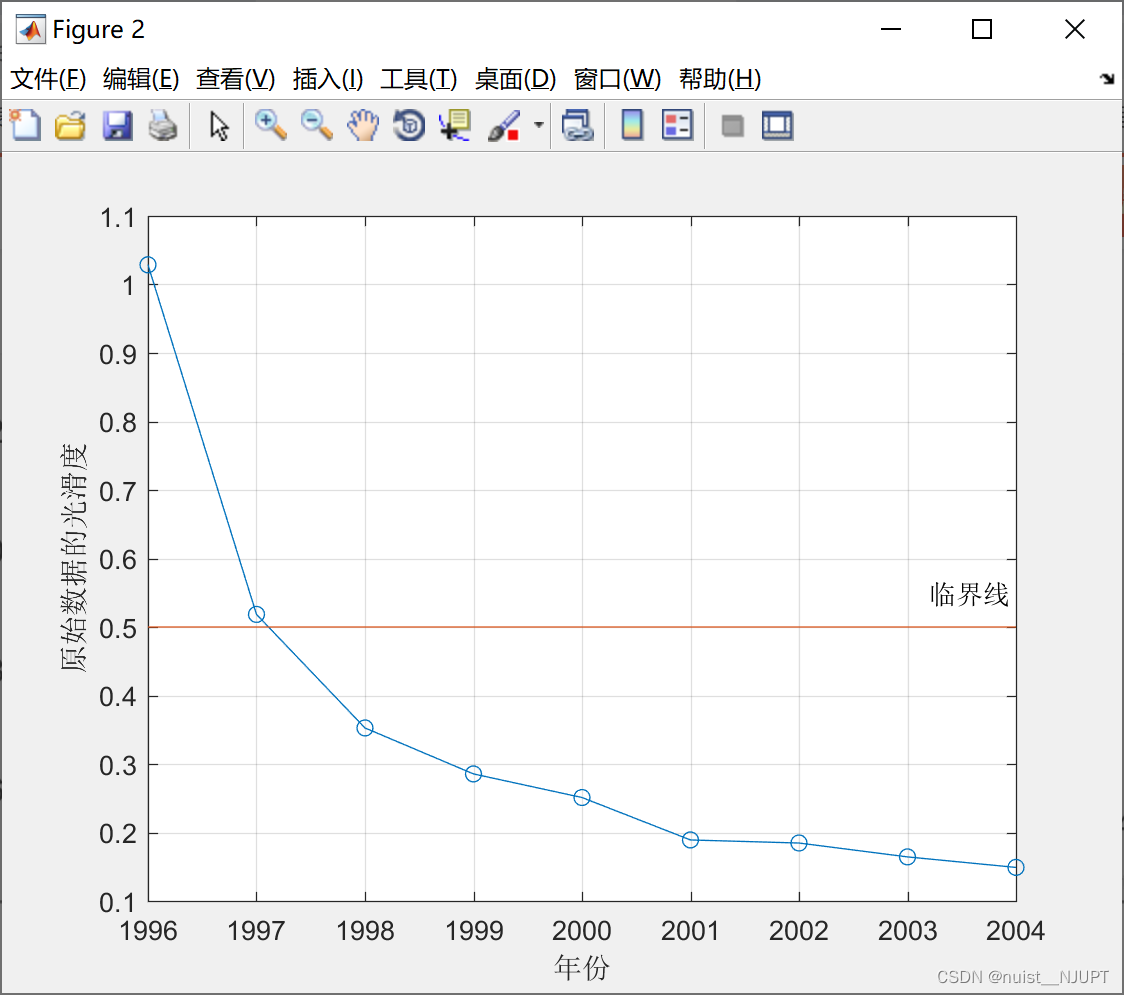

chart 4 Schematic diagram of the deviation degree between the predicted results of the three models of the test group and the actual real data , It can be found that the metabolic model works better , Closer to the true value , The sum of squares of errors is small .

The following diagram 5 It is residual error test and order ratio deviation test . It can be found that they are basically less than 0.1, All less than 0.2. The test passed .

The last is the future 10 Annual pollution forecast results , Give the number of gentlemen respectively , Fit the curve , And the curve predicted by grey model , It can be found that the prediction effect is good .

Four 、 Summary and analysis
For prediction topics , We can determine the model we need according to the following steps , First draw a picture and analyze , Then try different models in groups , Select a model to predict , Finally, draw the sequence diagram of the predicted data and the original data , See if the forecast trend is reasonable .

For when , We use the grey prediction model , Mainly consider the following three points , That is, the original data is non negative data measured by years , The data can pass the pre-test , The number of periods of data is the best thing 4~10 Episodic .

边栏推荐
- Under the pressure of technology, you can quickly get started with eth smart contract development, which will take you into the ETH world
- After 15 years of working on 21 types of hardware, where is Google?
- 赛芯电子冲刺科创板:拟募资6.2亿 实控人谭健为美国籍
- 牛客网:最小花费爬楼梯
- Half year inventory of new consumption in 2022: the industry is cold, but these nine tracks still attract gold
- 2022 Blue Bridge Cup group B - expense reimbursement - (linear dp| status DP)
- register_chrdev和cdev_init cdev_add用法区别
- Symantec electronic sprint technology innovation board: Tan Jian, the actual controller, is an American who plans to raise 620million yuan
- Bc1.2 PD protocol
- 2022蓝桥杯国赛B组-费用报销-(线性dp|状态dp)
猜你喜欢

什么是XR扩展现实,XR云串流平台有哪些

电子烟强制性国家标准GB 41700-2022发布 2022年10月1日起实施
![[BJDCTF2020]The mystery of ip|[CISCN2019 华东南赛区]Web11|SSTI注入](/img/c2/d6760826b81589781574aebff61f9a.png)
[BJDCTF2020]The mystery of ip|[CISCN2019 华东南赛区]Web11|SSTI注入

The new tea drinks are "dead and alive", but the suppliers are "full of pots and bowls"?

19:00 p.m. tonight, knowledge empowerment phase 2 live broadcast - control panel interface design of openharmony smart home project
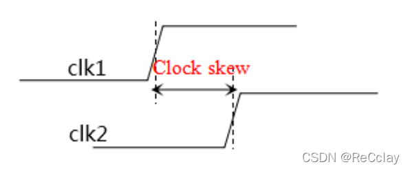
【Verilog基础】关于Clock信号的一些概念总结(clock setup/hold、clock tree、clock skew、clock latency、clock transition..)
Two methods for MySQL to open remote connection permission

大学生研究生毕业找工作,该选择哪个方向?

Open source STM32 USB-CAN project

Li Zexiang, a legendary Chinese professor, is making unicorns in batches

随机推荐
The new tea drinks are "dead and alive", but the suppliers are "full of pots and bowls"?
Halcon knowledge: regional topics [07]
“低代码”在企业数字化转型中扮演着什么角色?
Niuke.com: minimum cost of climbing stairs
大学生研究生毕业找工作,该选择哪个方向?
备战数学建模36-时间序列模型2
7 月 2 日邀你来TD Hero 线上发布会
360数科、蚂蚁集团等入选中国信通院“业务安全推进计划”成员单位
观测云与 TDengine 达成深度合作,优化企业上云体验
Niuke: how many different binary search trees are there
KDD 2022 | how far are we from the general pre training recommendation model? Universal sequence representation learning model unisrec for recommender system
Halcon knowledge: matrix topic [02]
What are the reasons for the errors reported by the Flink SQL CDC synchronization sqlserver
牛客网:有多少个不同的二叉搜索树
[time series database incluxdb] code example for configuring incluxdb+ data visualization and simple operation with C under Windows Environment
Carry two load balancing notes and find them in the future
备战数学建模33-灰色预测模型2
Log4j2 advanced use
详解Go语言中for循环,break和continue的使用
What role does "low code" play in enterprise digital transformation?