[Time series model] AR model (principle analysis + MATLAB code)

前言

Time series analysis methods include frequency domain analysis methods and time domain analysis methods.The time domain analysis method is to reveal the development law of time series from the perspective of sequence autocorrelation,The commonly used models are as follows：
自回归（AutoRegressive,AR）模型
移动平均（Moving Average,MA）模型
自回归移动平均（AutoRegressive Moving Average,ARMA）模型
差分自回归移动平均（AutoRegressive Integrated Moving Average,ARIMA）模型

一、ARAnalysis of the principle of the model

1.1 AR模型原理

A discrete time series for a set of observations$X$={ $x_1,x_2,...x_{N-1},x_N$},The value of each time series is not only related to the previous values,Also related to the resulting interference,Therefore, the time series can be represented by a linear difference equation：
$$x_i={\phi }_1{x}_{i-1}+{\phi }_2{x}_{i-2}+...+{\phi }_n{x}_{i-n}+a_i-{\theta }_1{a}_{i-1}-{\theta }_2{a}_{i-2}-...-{\theta }_m{a}_{i-m}$$
式中,$i=1,2,...,N.$,$a_i为模型残差$.
When the moving average coefficient${\theta }_j=0(j=1,2,...,m.)$时,That is, there is no moving average part,上式变为：
$$x_i={\phi }_1{x}_{i-1}+{\phi }_2{x}_{i-2}+...+{\phi }_n{x}_{i-n}+a_i$$
Call this expression $n$阶自回归模型$AR(n)$.

1.2 模型的参数估计

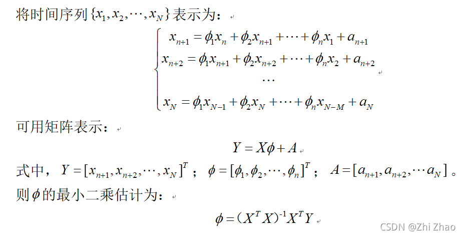
ARThe parameter estimation of the model is based on the known observational data ,Estimate constant coefficients according to a method ${\phi }_i$ 和 ${\sigma }_a^2$ 这 $n+1$ 个参数.There are two types of parameter estimation methods：直接法和间接法.Direct methods include least squares estimation methods、解Yuler-WalkerEquations etc;Indirect methods includeLUD法、Burg法等.Due to the high accuracy of parameter estimation using the least squares method、It has the advantages of simplicity and unbiased estimation,Therefore, the least squares method is used to solve itAR模型参数.

1.3 The order method of the model

ARThe determination of the model order has a great influence on the accuracy of the model prediction,When the model order is less than the optimal model order,Time series can have an overly smooth effect,As a result, the amount of information it carries is greatly reduced;When the model order is greater than the optimal model order,Some noise still exists,This increases the error of the model fitting,影响预测的准确性.
Model ordering is usually based on the closeness of the model fitting to the original data to determine the use of the best criterion function,When modeling, the quality of the model is determined according to the value of the criterion function.

（1）AIC

赤池信息量准则（Akaike Information Criterion,AIC）It is the Japanese scholar Akaike Hiroshi1973年提出,并成功应用于ARModel ordering and selection.This criterion is based on the concept of entropy,It can measure the goodness of model fit.Akaike Hiroji pointed outA time series can be divided into several locally stable periods,Available every time period AR模型来拟合.

AIC准则函数定义为：
$$AIC(k)=2k-2ln(L)$$
其中,$k$是参数的数量,is the order of the model;$L$为似然函数.

（2）BIC

当训练模型时,增加参数的数量,That is to increase the complexity of the model,Thereby increasing the likelihood function,However, the model can also overfit.为了解决这个问题,Schwarz 于1978The Bayesian Information Criterion was proposed in 2007（Bayes Information Criterion,BIC）,Also known as Bayesian Information Criterion.
BIC准则函数定义为：
$$BIC(k)=kln(n)-2ln(L)$$
其中,$k$是参数的数量,is the order of the model;$n$为样本个数;$L$为似然函数.
$kln(n)$为惩罚项,在样本数量较多的情况下,It can effectively prevent the problem of excessive model complexity caused by excessive model accuracy,The phenomenon of the curse of dimensionality is avoided.

二、MATLAB代码

1、Call the linear predictor functionlpc计算模型的参数

clc;
clear;
close all;

randn('state',0); 
noise = randn(50000,1);  % Normalized white Gaussian noise
x = filter(1,[1 1/2 1/3 1/4],noise);
x = x(45904:50000);
a = lpc(x,3);
est_x = filter([0 -a(2:end)],1,x);  % Estimated signal
e = x - est_x;                      % Prediction error
[acs,lags] = xcorr(e,'coeff');      % ACS of prediction error

%   Compare the predicted signal to the original signal
figure;
plot(1:97,x(4001:4097),1:97,est_x(4001:4097),'--');
title('Original Signal vs. LPC Estimate');
xlabel('Sample Number'); ylabel('Amplitude'); grid on;
legend('Original Signal','LPC Estimate')

%   Look at the autocorrelation of the prediction error.
figure;
plot(lags,acs); 
title('Autocorrelation of the Prediction Error');
xlabel('Lags'); ylabel('Normalized Value'); grid on;

2、利用 Yule-Walker to calculate the parameters of the model

clc;
clear;
close all;

% Estimate model order using decay of reflection coefficients.
rng default;
y=filter(1,[1 -0.75 0.5],0.2*randn(1024,1));
% Create AR(2) process
[ar_coeffs,NoiseVariance,reflect_coeffs] = aryule(y,10);

% Fit AR(10) model
stem(reflect_coeffs);
axis([-0.05 10.5 -1 1]);
title('Reflection Coefficients by Lag');
xlabel('Lag');ylabel('Reflection Coefficent');

3、利用 Burg to calculate the parameters of the model

clc;
clear;
close all;

%  Estimate input noise variance for AR(4) model.
A = [1 -2.7607 3.8106 -2.6535 0.9238]; 
% Generate noise standard deviations
rng default;
noise_stdz = rand(1,50)+0.5;

% Generate column vectors that have corresponding standard deviation
x = bsxfun(@times,noise_stdz,randn(1024,50));

% filter each column using the AR model.
y = filter(1,A,x);

% Compute the estimated coefficients and deviations for each column
[ar_coeffs,NoiseVariance]=arburg(y,4);

% Display the mean value of each estimated polynomial coefficient
estimatedA = mean(ar_coeffs);

% Compare actual vs. estimated variances
plot(noise_stdz.^2,NoiseVariance,'k*');
xlabel('Input Noise Variance');
ylabel('Estimated Noise Variance');

三、AR相关论文

（1）Recognition method of arrival time of rock acoustic emission signal based on de-noising：In the study of time difference location of rock acoustic emission source, Signal arrival time is important information.Rock acoustic emission signals are complex, Contains a lot of impulse interference and random noise, Arrival times are poorly readable.针对以上问题, Firstly, median filtering and singular value decomposition are performed on the original acoustic emission signal, Eliminate some impulse interference and random noise; Secondly, wavelet packet decomposition and soft threshold denoising are performed, The main components of the signal are preserved, 提高信噪比, Improve readability of arrival times; Finally, a time series model of signal and noise is combined( AutoＲegressive, AＲ 模型) , 第 1 time to calculate the Akaike Information Criterion K 值( Akaike Information Criterion, AIC( K) 值) , Get the arrival time window, in this window 2 次计算 AIC( K) 值, The automatic identification of arrival time is realized, Computation under the entire signal sequence is avoidedARThe order and degree of the model.

（2）基于CEEMDAN和ARResearch on the feature extraction method of rock mass acoustic emission signal：The acoustic emission signal for rocks is non-stationary、It is difficult to effectively extract feature parameters due to the complexity of features,An empirical decomposition algorithm based on adaptive complete ensemble is proposed(CEEMDAN)和AR模型的特征提取方法,Taking red sandstone as the research object,用CEEMDANDecompose the signal of its rupture phase,Use the correlation coefficient method to select effectiveIMF分量,And perform energy normalization processing,to eliminate the influence of other factors on the model.By calculating the signal at each stageAR模型的AIC值,Build the best order modelAR(5),The accuracy of the model is verified by comparative experiments,并将提取的５阶ARModel coefficients as eigenvectors,It provides a basis and method for the subsequent prediction of rock instability.

参考文献：

[1] Xian Xiaodong,袁 双,Ji Songlin. Recognition method of arrival time of rock acoustic emission signal based on de-noising[J]. 煤炭学报, 2015, 40(S1) : 100-106.
[2] Dai Congcong, 罗小燕, Shao Fan, Huang Xiaoyong, Xu Sixiang.基于CEEMDAN和ARResearch on the feature extraction method of rock mass acoustic emission signal[J]. Chemical minerals and processing, 2018, 47(06) : 20-24.