当前位置：网站首页>Machine learning notes - supervised learning memo list

Machine learning notes - supervised learning memo list

2022-06-13 06:36:00 【Sit and watch the clouds rise】

One 、 Introduction to supervised learning

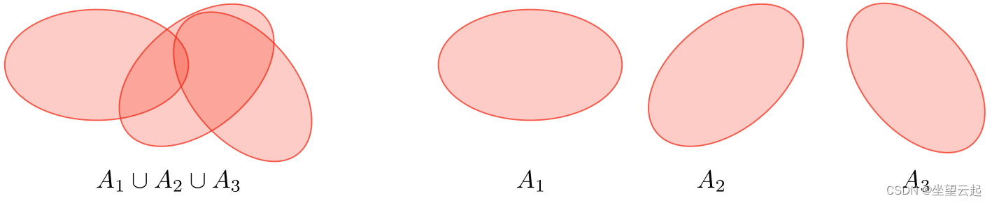
Given a set of data points $\{x^{(1)}, ..., x^{(m)}\}$ Associate to a set of results $\{y^{(1)}, ..., y ^{(m)}\}$ , We want to build a classifier , Learn how to learn from forecast .

1、 Forecast type

The following table summarizes the different types of forecasting models ：

2、 Model type

The following table summarizes the different models ：

Two 、 Symbols and general concepts

1、Hypothesis

This assumption is marked as $h_\theta$ And the model we chose . For a given input data $x^{(i)}$ , The prediction output of the model is $h_\theta(x^{(i)})$ .

2、Loss function

The loss function is a function $L:(z,y)\in\mathbb{R}\times \longmapsto L(z,y)\in\mathbb{R}$ , It will be compared with the real data value The corresponding predicted value As input , And output their differences . The following table summarizes the common loss functions ：

3、Cost function

cost function It is usually used to evaluate the performance of the model , Its loss function The definition is as follows ：

$\boxed{J(\theta)=\sum_{i=1}^mL(h_\theta(x^{(i)}), y^{(i)})}$

4、Gradient descent

By paying attention to $\alpha\in\mathbb{R}$ Learning rate , The updating rule of gradient descent is a function of learning rate and cost Shown by the following ：

$\boxed{\theta\longleftarrow\theta-\alpha\nabla J(\theta)}$

remarks ： Stochastic gradient descent （SGD） Is to update the parameters according to each training sample , Batch gradient descent is performed on a batch of training samples .

5、Likelihood

The given parameters $\theta$ Model of $L(\theta)$ The likelihood of is used to find the optimal parameters by likelihood maximization $\theta$ . We have ：

$\boxed{\theta^{\textrm{opt}}=\underset{\theta}{\textrm{arg max }}L(\theta)}$

remarks ： In practice , We use log likelihood, which is easier to optimize $\ell(\theta)=\log(L(\theta))$ .

6、Newton's algorithm

Newton's algorithm is a method of solving $\theta$ The numerical method of , bring $\ell'(\theta)=0$ . The update rules are as follows ： $\boxed{\theta\leftarrow\theta-\frac{\ell'(\theta)}{\ell''(\theta)}}$

remarks ： Multidimensional generalization , Also known as Newton-Raphson Method , There are the following update rules ：

$\theta\leftarrow\theta-\left(\nabla_\theta^2\ell(\theta)\right)^{-1}\nabla_\theta\ell(\theta)$

3、 ... and 、 Linear model

1、 Linear regression

Let's assume here that $y|x;\theta\sim\mathcal{N}$

（1）Normal equations

By paying attention to the design matrix , Minimize the cost function $\theta$ The value of is a closed form solution , bring ：

$\boxed{\theta=(X^TX)^{-1}X^Ty}$

（2）LMS algorithm

By paying attention to α Learning rate , Least mean square (LMS) Algorithm to m Update rules for training sets of data points , Also known as Widrow-Hoff Learning rule , As shown below ：

$\boxed{\forall j,\quad \theta_j \leftarrow \theta_j+\alpha\sum_{i=1}^m\left[y^{(i)}-h_\theta(x^{(i)})\right]x_j^{(i)}}$

remarks ： The update rule is a special case of gradient rise .

（3）LWR

Local weighted regression , Also known as LWR, Is a variant of linear regression , It passes through $w^{(i)}(x)$ Each training sample is weighted in its cost function , It's made up of parameters $\tau \in\mathbb{R}$ Defined as ：

$\boxed{w^{(i)}(x)=\exp\left(-\frac{(x^{(i)}-x)^2}{2\tau^2}\right)}$

2、 Classification and logical regression

（1）Sigmoid function

sigmoid function , Also known as logical functions , The definition is as follows ： $\forall z\in\mathbb{R},\quad\boxed{g(z)=\frac{1}{1+e^{-z}}\in[0,1]}$

（2）Logistic regression

Let's assume here that $y|x;\theta\sim\textrm{Bernoulli} (\phi)$ . We have the following forms ：

$\boxed{\phi=p(y=1|x;\theta)=\frac{1}{1+\exp(-\theta^Tx)}=g(\theta^Tx)}$

remarks ： There is no closed form solution for logistic regression .

（3）Softmax regression

When there is more than 2 Result categories ,softmax Return to , Also called multi class logistic regression , Used to generalize logistic regression . By convention , We set up $\theta_K=0$ , This makes every class Bernoulli parameter of $\phi_i$ by ：

$\boxed{\displaystyle\phi_i=\frac{\exp(\theta_i^Tx)}{\displaystyle\sum_{j=1}^K\exp(\theta_j^Tx)}}$

3、 Generalized linear model

（1）Exponential family

If a kind of distribution can use natural parameters （ Also known as canonical arguments or link functions ）、 $\eta$ 、 Sufficient statistics T(y) And logarithm , It belongs to log-partition function $a(\eta)$ as follows ：

$\boxed{p(y;\eta)=b(y)\exp(\eta T(y)-a(\eta))}$

remarks ： We often have T(y)=y . Besides , $\exp(-a(\eta))$ It can be regarded as a standardized parameter , It will ensure that the sum of the probabilities is 1.

The following table summarizes the most common exponential distributions ：

（2）Assumptions of GLMs

Generalized linear model (GLM) To predict random variables As $x\in\mathbb{R}^{n+1}$ Function of , And depends on the following 3 A hypothesis ：

(1) $\quad\boxed{y|x;\theta\sim\textrm{ExpFamily}(\eta)}$ (2) $\quad\boxed{h_\theta(x)=E[y|x;\theta]}$ (3) $\boxed{\eta=\theta^Tx}$

remarks ： Ordinary least square method and logistic regression are special cases of generalized linear model .

Four 、 Support vector machine

The goal of support vector machine is to find the line with the minimum distance and the maximum distance from the line .

1、Optimal margin classifier

Best margin classifier That's true ： $\boxed{h(x)=\textrm{sign}(w^Tx-b)}$ , among $(w, b)\in\mathbb{R}^n\times\mathbb{R}$ Is the solution of the following optimization problem ： $\boxed{\min\frac{1}{2}||w||^2}\quad\quad\textrm{such that }\quad \boxed{y^{(i)}(w^Tx^{(i)}-b)\geqslant1}$

remarks ： The decision boundary is defined as $\boxed{w^Tx-b=0}$

2、Hinge loss

hinge loss be used for SVM Set up , The definition is as follows ： $\boxed{L(z,y)=[1-yz]_+=\max(0,1-yz)}$

3、Kernel

Given a feature map $\phi$ , We will use the kernel The definition is as follows ： $\boxed{K(x,z)=\phi(x)^T\phi(z)}$

In practice , from $K(x,z)=\exp\left(-\frac{||x-z||^2}{2\sigma^2}\right)$ Defined kernel It is called Gaussian kernel , More commonly used .

remarks ： We say we use “ Kernel techniques ” To use the kernel to compute cost functions , Because we don't really need to know the explicit mapping $\phi$ , This is usually very complicated . contrary , Just the value K(x,z) .

4、Lagrangian

We will Lagrange $\mathcal{L}(w,b)$ The definition is as follows ： $\boxed{\mathcal{L}(w,b)=f(w)+\sum_{i=1}^l\beta_ih_i(w)}$

remarks ： coefficient $\beta_i$ It is called Lagrange multiplier .

5、 ... and 、 Generative learning

The generation model first attempts to estimate P(x|y) To learn how to generate data , Then we can use Bayesian estimation P(y|x) The rules .

1、Gaussian Discriminant Analysis

（1）Setting

Gaussian discriminant analysis hypothesis and x|y=0 and x|y=1 That's true ：
(1) $\quad\boxed{y\sim\textrm{Bernoulli}(\phi)}$ (2) $\quad\boxed{x|y=0\sim\mathcal{N}(\mu_0,\Sigma)}$ (3) $\quad\boxed{x|y=1\sim\mathcal{N}(\mu_1,\Sigma)}$

（2）Estimation

The following table summarizes the estimates we found when maximizing likelihood ：

2、Naive Bayes

（1）Assumption

Naive Bayesian model assumes that the characteristics of each data point are independent ：

$\boxed{P(x|y)=P(x_1,x_2,...|y)=P(x_1|y)P(x_2|y)...=\prod_{i=1}^nP(x_i|y)}$

（2）Solutions

Maximizing log likelihood gives the following solution ：

$\boxed{P(y=k)=\frac{1}{m}\times\#\{j|y^{(j)}=k\}}\quad\textrm{ and }\quad\boxed{P(x_i=l|y=k)=\frac{\#\{j|y^{(j)}=k\textrm{ and }x_i^{(j)}=l\}}{\#\{j|y^{(j)}=k\}}}$

$k\in\{0,1\} , l\in[\![1,L]\!]$

remarks ： Naive Bayes is widely used in text classification and spam detection .

6、 ... and 、 Tree based and integrated approach

These methods can be used for regression and classification problems .

1、CART

Classification and regression trees （CART）, Commonly known as decision tree , Can be expressed as a binary tree . Their advantage is that they are easy to explain .

2、Random forest

It is a tree based technology , It uses a large number of decision trees constructed from randomly selected feature sets . Contrary to a simple decision tree , It is highly unexplainable , But its generally good performance makes it a popular algorithm . remarks ： Random forest is an integrated method .

3、Boosting

The idea of the lifting method is to combine several weak learners into a stronger one . The main conclusions are as follows ：

Adaptive boosting	Gradient boosting
• High weights are put on errors to improve at the next boosting step • Known as Adaboost	• Weak learners are trained on residuals • Examples include XGBoost

7、 ... and 、 Other nonparametric methods

1、k-nearest neighbors

k- Nearest neighbor algorithm , Often referred to as k-NN, It's a nonparametric method , The response of data points is determined by the k The nature of a neighbor determines . It can be used for classification and regression settings .

notes ： Parameters k The higher the , The bigger the deviation , Parameters k The lower the , The higher the variance is. .

8、 ... and 、 Learning theory

1、Union bound

Make A_1, ..., A_k by k Events . We have ： $\boxed{P(A_1\cup ...\cup A_k)\leqslant P(A_1)+...+P(A_k)}$

2、Hoeffding inequality

Make Z_1, .., Z_m From the parameters $\phi$ Extracted from Bernoulli distribution m iid Variable . set up $\widehat{\phi}$ For their sample mean , also $\gamma>0$ Fix . We have ： $\boxed{P(|\phi-\widehat{\phi}|>\gamma)\leqslant2\exp(-2\gamma^2m)}$

remarks ： This inequality is also called Chernoff bound .

3、Training error

For a given classifier h, We define training error $\widehat{\epsilon}(h)$ , Also known as empirical risk or empirical error , as follows ：

$\boxed{\widehat{\epsilon}(h)=\frac{1}{m}\sum_{i=1}^m1_{\{h(x^{(i)})\neq y^{(i)}\}}}$

4、Probably Approximately Correct (PAC)

PAC It's a framework , Many results of learning theory are proved under this framework , And has the following set of assumptions ：

The training set and the test set follow the same distribution

Training samples are drawn independently

5、Shattering

Given a set $S=\{x^{(1)},...,x^{(d)}\}$ And a set of classifiers $\mathcal{H}$ , We said $\mathcal{H}$ about If for any set of labels $\{y^{(1)}, ..., y^{(d)}\}$ , We have ： $\boxed{\exists h\in\mathcal{H}, \quad \forall i\in[\![1,d]\!],\quad h(x^{(i)})=y^{(i)}}$

6、Upper bound theorem

Make $\mathcal{H}$ Is a finite hypothetical class , bring $|\mathcal{H}|=k$ And make $\delta$ And sample size Is constant . then , At least $1-\delta$ Probability , We have ：

$\boxed{\epsilon(\widehat{h})\leqslant\left(\min_{h\in\mathcal{H}}\epsilon(h)\right)+2\sqrt{\frac{1}{2m}\log\left(\frac{2k}{\delta}\right)}}$

7、VC dimension

Given an infinite hypothetical class $\mathcal{H}$ Of Vapnik-Chervonenkis (VC) dimension , Write it down as $\textrm{VC} (\mathcal{H})$ Be being The size of the largest set of fragments .

notes ： ${\small\mathcal{H}=\{\textrm{set of linear classifiers in 2 dimensions}\}}$ Of VC Dimension is 3.

8、Theorem (Vapnik)

set up $\mathcal{H}$ , $\textrm{VC}(\mathcal{H})=d$ and It's the number of training samples . At least $1-\delta$ Probability , We have ：

$\boxed{\epsilon(\widehat{h})\leqslant \left(\min_{h\in\mathcal{H}}\epsilon(h)\right) + O\left(\sqrt{\frac{d}{m}\log\left(\frac{m}{d}\right)+\frac{1}{m}\log\left(\frac{1}{\delta}\right)}\right)}$