当前位置:网站首页>NBA player analysis
NBA player analysis
2022-07-02 15:26:00 【Little doll】
List of articles
- 1. get data
- 2. Data analysis
- 3. Team data analysis
- 3.1 Team salary ranking
- 3.2 According to the team By age group , The number of players on the list is the same , Then arrange them in descending order according to the efficiency value
- 3.3 Rank according to the comprehensive strength of the team
- 3.4 Use box diagram and violin diagram for data analysis
1. get data
data=pd.read_csv("./data/nba_2017_nba_players_with_salary.csv")
data.head(10)

2. Data analysis
2.1 Data relevance
data_cor = data.loc[:, ['RPM', 'AGE', 'SALARY_MILLIONS', 'ORB', 'DRB', 'TRB',
                       'AST', 'STL', 'BLK', 'TOV', 'PF', 'POINTS', 'GP', 'MPG', 'ORPM', 'DRPM']]
data_cor.head()

#  Get the size comparison of the data correlation in the table
corr=data_cor.corr()
#h Get the correlation between the two columns of data
corr.head()

plt.figure(figsize=(20,8),dpi=100)
sns.heatmap(corr,square=True,linewidths=0.1,annot=True)  # According to relevance   Get the thermodynamic diagram of two columns of data

2.2 Basic data ranking analysis
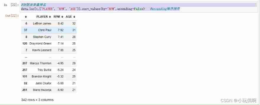
# Rank according to efficiency value
data.loc[:,["PLAYER", "RPM", "AGE"]].sort_values(by="RPM",ascending=False)   #ascending null
#  Rank by player salary
data.loc[:,["PLAYER", "RPM", "SALARY_MILLIONS"]].sort_values(by="SALARY_MILLIONS",ascending=False)   #ascending null

2.3 Seaborn Three commonly used data visualization methods
2.3.1 Univariate
#  utilize seaborn Medium distplot Draw a picture to see the salary of players 、 Efficiency value 、 The distribution of age
sns.set_style("darkgrid")#  Set the style of the image
plt.figure(figsize=(10,10))  # Set the size of the canvas
plt.subplot(3,1,1)  # Usage method :subplot(m,n,p) perhaps subplot(m n p). subplot It's a tool for drawing multiple pictures on one plane . among ,m It's a graph arrangement m That's ok ,n The graphs are arranged in n Column , That is the whole figure There is n The two graphs are arranged in a row , altogether m That's ok , If m=2 That is to say 2 Line graph .p Show the location of the diagram ,p=1 Represents the first position from left to right, top to bottom .
sns.distplot(data["SALARY_MILLIONS"])
plt.ylabel("salary")

plt.subplot(3,1,2)  # Usage method :subplot(m,n,p) perhaps subplot(m n p). subplot It's a tool for drawing multiple pictures on one plane . among ,m It's a graph arrangement m That's ok ,n The graphs are arranged in n Column , That is the whole figure There is n The two graphs are arranged in a row , altogether m That's ok , If m=2 That is to say 2 Line graph .p Show the location of the diagram ,p=1 Represents the first position from left to right, top to bottom .
sns.distplot(data["RPM"])
plt.ylabel("RPM")

plt.subplot(3,1,3)  # Usage method :subplot(m,n,p) perhaps subplot(m n p). subplot It's a tool for drawing multiple pictures on one plane . among ,m It's a graph arrangement m That's ok ,n The graphs are arranged in n Column , That is the whole figure There is n The two graphs are arranged in a row , altogether m That's ok , If m=2 That is to say 2 Line graph .p Show the location of the diagram ,p=1 Represents the first position from left to right, top to bottom .
sns.distplot(data["AGE"])
plt.ylabel("AGE")

2.3.2 Bivariate
sns.jointplot(data.AGE,data.SALARY_MILLIONS,kind="hex")

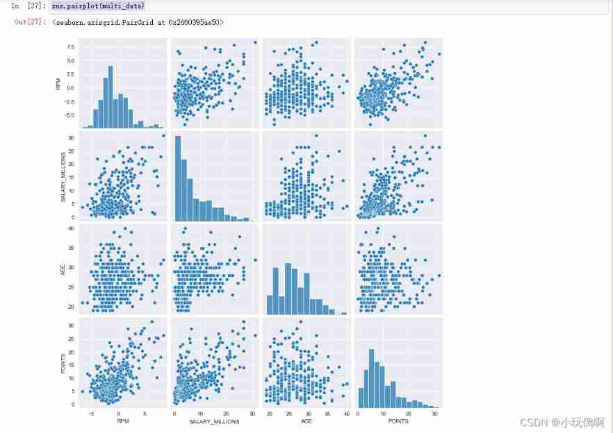
2.3.3 Multivariable
multi_data = data.loc[:, ['RPM','SALARY_MILLIONS','AGE','POINTS']]
multi_data.head()

sns.pairplot(multi_data)
2.3.4 Some visualization practices of derived variables - Take age as an example
def age_cut(df):
    ''' Age division '''
    if df.AGE<=24:
        return "young"
    elif df.AGE>=30:
        return "old"
    else:
        return "best"

data["age_cut"]=data.apply(lambda x:age_cut(x),axis=1)
#apply effect : The first parameter is the pointer of the custom function , Pass the function in , then apply The function will data A line in is passed into the function as a parameter ,axis=1  Represents a line by line calculation
data.head()

#  Easy to count
data["cut"]=1
data.loc[data.age_cut=="best"].SALARY_MILLIONS.head()

#  Analyze player salary and efficiency based on age
sns.set_style("darkgrid")
plt.figure(figsize=(10,10),dpi=100)
plt.title("RPM and Salary")

x1=data.loc[data.age_cut=="old"].SALARY_MILLIONS
y1=data.loc[data.age_cut=="old"].RPM
plt.plot(x1,y1,"^")

x2=data.loc[data.age_cut=="best"].SALARY_MILLIONS
y2=data.loc[data.age_cut=="best"].RPM
plt.plot(x2,y2,"^")

x3=data.loc[data.age_cut=="young"].SALARY_MILLIONS
y3=data.loc[data.age_cut=="young"].RPM
plt.plot(x3,y3,".")

multi_data2 = data.loc[:, ['RPM','POINTS','TRB','AST','STL','BLK','age_cut']]
sns.pairplot(multi_data2,hue="age_cut")  # hue Continue to display in color according to this column

3. Team data analysis
3.1 Team salary ranking
data.groupby(by="age_cut").agg({
    "SALARY_MILLIONS":np.mean})  # Group by age , Then aggregate according to the average

data_team=data.groupby(by="TEAM").agg({
    "SALARY_MILLIONS":np.mean})  # Group according to the team , Then aggregate according to the average
data_team.sort_values(by="SALARY_MILLIONS",ascending=False).head()#  Sort by salary in descending order  ascending=False For the descending order

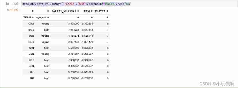
3.2 According to the team By age group , The number of players on the list is the same , Then arrange them in descending order according to the efficiency value
data_RMP=data.groupby(by=["TEAM","age_cut"]).agg({
    "SALARY_MILLIONS":np.mean,"RPM":np.mean,"PLAYER":np.size})
data_RMP.head()

data_RMP.sort_values(by=["PLAYER","RPM"],ascending=False).head(10)
3.3 Rank according to the comprehensive strength of the team
data_rpm2=data.groupby(by=["TEAM"],as_index=False).agg({
    "SALARY_MILLIONS":np.mean,
                                                        "RPM":np.mean,
                                                        "PLAYER":np.size,
                                                        "POINTS":np.mean,
                                                        "eFG%":np.mean,
                                                        "MPG":np.mean,
                                                        "AGE":np.mean})
data_rpm2.head()

data_rpm2.sort_values(by="RPM",ascending=False)

3.4 Use box diagram and violin diagram for data analysis
sns.set_style("whitegrid")#  Set the style of the drawing board
# Get the corresponding data
data_team2=data[data.TEAM.isin(['GS','CLE','SA','LAC','OKC','UTAH',"CHA",'TOR','NO','BOS'])]
data_team2.head()

# Make corresponding drawings
plt.figure(figsize=(20,10))# Set the size of the sketchpad
plt.subplot(3,1,1)
sns.boxplot(x="TEAM",y="SALARY_MILLIONS",data=data_team2)

plt.subplot(3,1,2)
sns.boxplot(x="TEAM",y="AGE",data=data_team2)

plt.subplot(3,1,3)
sns.boxplot(x="TEAM",y="MPG",data=data_team2)

# Draw a picture of the violin
sns.set_style("whitegrid")
plt.figure(figsize=(20,10))
plt.subplot(3,1,1)
sns.violinplot(x="TEAM",y="3P%",data=data_team2)

plt.subplot(3,1,2)
sns.violinplot(x="TEAM",y="eFG%",data=data_team2)

plt.subplot(3,1,3)
sns.violinplot(x="TEAM",y="POINTS",data=data_team2)

边栏推荐
- Why can't programmers who can only program become excellent developers?
- 04.进入云原生后的企业级应用构建的一些思考
- How to test tidb with sysbench
- 14_Redis_乐观锁
- Practical debugging skills
- 20_Redis_哨兵模式
- Tidb environment and system configuration check
- Equipped with Ti am62x processor, Feiling fet6254-c core board is launched!
- Pytorch 保存tensor到.mat文件
- 08_ 串
猜你喜欢
基于RZ/G2L | OK-G2LD-C开发板存储读写速度与网络实测

16_ Redis_ Redis persistence
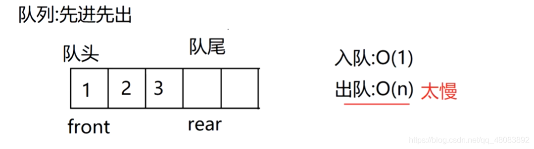
05_队列
CodeCraft-22 and Codeforces Round #795 (Div. 2)D,E
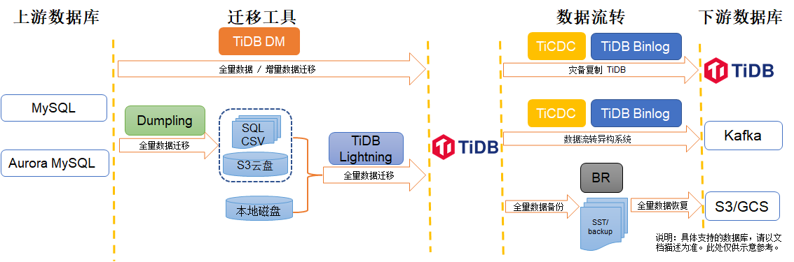
TiDB数据迁移工具概览

08_ strand
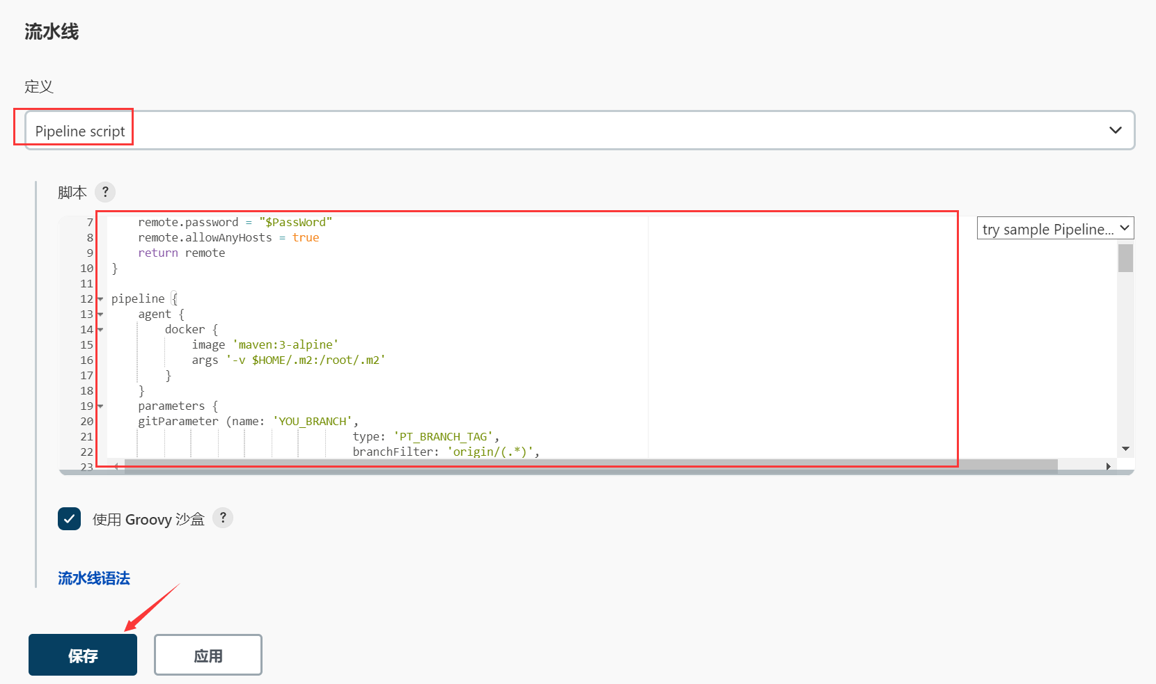
Jenkins Pipeline 应用与实践
How does the computer set up speakers to play microphone sound

6.12 企业内部upp平台(Unified Process Platform)的关键一刻
![[C language] explain the initial and advanced levels of the pointer and points for attention (1)](/img/61/1619bd2e959bae1b769963f66bab4e.png)
[C language] explain the initial and advanced levels of the pointer and points for attention (1)
随机推荐
Principles, language, compilation, interpretation
18_Redis_Redis主从复制&&集群搭建
语义分割学习笔记(一)
如何用 Sysbench 测试 TiDB
17_ Redis_ Redis publish subscription
03_ Linear table_ Linked list
Application and practice of Jenkins pipeline
记一次面试
08_ strand
QML pop-up frame, customizable
13_Redis_事务
Common English abbreviations for data analysis (I)
FPGA - 7系列 FPGA内部结构之Clocking -03- 时钟管理模块(CMT)
Equipped with Ti am62x processor, Feiling fet6254-c core board is launched!
如何对 TiDB 进行 TPC-C 测试
CodeCraft-22 and Codeforces Round #795 (Div. 2)D,E
How to test tidb with sysbench
Dragonfly low code security tool platform development path
AtCoder Beginner Contest 254
LeetCode_ String_ Simple_ 412.Fizz Buzz