Scanpy (VI) analysis and visualization of spatial transcriptome data

This article demonstrates how to Scanpy Using spatial transcriptome data in （spatial transcriptomics data）, First , We focus on 10x Genomics Visium data, Last , We are MERFISH Technology provides an example of spatial transcription data analysis .

---

At present, the technology of spatial transcriptome has not reached the level of single cell , A general spatial location spots There are multiple cells on the ,10X Genomics Visum It's usually 1-10 Cells , Spatial transcriptomics can provide spatial location , But the resolution can not reach the single cell level , Single cell transcriptome resolution can reach single cell resolution , But there is no spatial location information , Therefore, if the spatial transcriptome is combined with the single-cell transcriptome , Then there is the spatial location information , The single cell resolution is reached , This provides a powerful tool for the scientific community , Greatly improve the organization of organisms 、 The resolution and accuracy of organ studies .

---

We import scanpy Tools ：

import scanpy as sc
import pandas as pd
import matplotlib.pyplot as plt
import seaborn as sns

sc.logging.print_versions()
sc.set_figure_params(facecolor="white", figsize=(8, 8))
sc.settings.verbosity = 3

""" anndata 0.8.0 scanpy 1.9.1 """

Reading data

We will use human lymph nodes （human lymphnode） Of Visium Spatial transcriptomics data set , This data set is published in 10x genomics website：link;

function datasets.visium_sge() from 10x Genomics Download datasets , And returns a matrix containing the count counts And spatial coordinates spatital coordinates Of AnnData object .

adata = sc.datasets.visium_sge(sample_id="V1_Human_Lymph_Node")
adata.var_names_make_unique()

adata
""" AnnData object with n_obs × n_vars = 4035 × 36601 obs: 'in_tissue', 'array_row', 'array_col' var: 'gene_ids', 'feature_types', 'genome' uns: 'spatial' obsm: 'spatial' """

We will use pp.calculate_qc_metrics And based on mitochondria read counts Calculation QC indicators .

#  Save the mitochondrial genome as an annotation  var.mt
adata.var["mt"] = adata.var_names.str.startswith("MT-")
adata.var["mt"]
""" MIR1302-2HG False ... AC007325.2 False Name: mt, Length: 36601, dtype: bool """

#  Calculate the index , qc Of var choice  var.mt
sc.pp.calculate_qc_metrics(adata, qc_vars=["mt"], inplace=True)

adata
""" AnnData object with n_obs × n_vars = 4035 × 36601 obs: 'in_tissue', 'array_row', 'array_col', 'n_genes_by_counts', 'log1p_n_genes_by_counts', 'total_counts', 'log1p_total_counts', 'pct_counts_in_top_50_genes', 'pct_counts_in_top_100_genes', 'pct_counts_in_top_200_genes', 'pct_counts_in_top_500_genes', 'total_counts_mt', 'log1p_total_counts_mt', 'pct_counts_mt' var: 'gene_ids', 'feature_types', 'genome', 'mt', 'n_cells_by_counts', 'mean_counts', 'log1p_mean_counts', 'pct_dropout_by_counts', 'total_counts', 'log1p_total_counts' uns: 'spatial' obsm: 'spatial' """

review Scanpy( 3、 ... and ) Handle 3k PBMCs Parallel clustering The content in , We can understand the meaning of some quality ：

• n_genes_by_counts： In every cell , Number of genes expressed ;
• total_counts： Total gene count per cell （ Total meter volume ）;
• pct_counts_mt： In every cell , The percentage of mitochondrial gene expression in all gene expression of the cell ;

QC and preprocessing

We according to the total_counts and n_genes_by_counts Do some basic filtering . We first visualize these quality indicators as histograms ：

fig, axs = plt.subplots(1, 4, figsize=(15, 4))
sns.distplot(adata.obs["total_counts"], kde=False, ax=axs[0])
sns.distplot(adata.obs["total_counts"][adata.obs["total_counts"] < 10000], kde=False, bins=40, ax=axs[1])
sns.distplot(adata.obs["n_genes_by_counts"], kde=False, bins=60, ax=axs[2])
sns.distplot(adata.obs["n_genes_by_counts"][adata.obs["n_genes_by_counts"] < 4000], kde=False, bins=60, ax=axs[3])

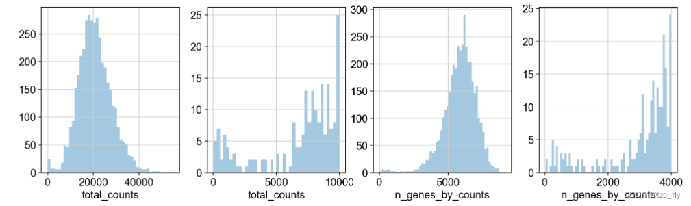
The second graph is the first graph in 0 To 10000 Visualization of intervals ,total_counts Represents the total gene expression of a cell . The fourth graph is the third graph in 0 To 4000 Visualization ,n_genes_by_counts Represents a cell , Number of genes expressed . Be careful , The counting matrix is 4035×36601.

Through the above visualization results , We reserve the total_counts stay 5000 To 35000 The cells , next step , We keep mitochondrial genes pct_counts_mt The proportion is less than 20% The cells . Last , Do genetic filtering ：

sc.pp.filter_cells(adata, min_counts=5000)
sc.pp.filter_cells(adata, max_counts=35000)
adata = adata[adata.obs["pct_counts_mt"] < 20]
print(f"#cells after MT filter: {
      adata.n_obs}")
sc.pp.filter_genes(adata, min_cells=10)

""" filtered out 44 cells that have less than 5000 counts filtered out 130 cells that have more than 35000 counts #cells after MT filter: 3861 filtered out 16916 genes that are detected in less than 10 cells """

adata
""" AnnData object with n_obs × n_vars = 3861 × 19685 obs: 'in_tissue', 'array_row', 'array_col', 'n_genes_by_counts', 'log1p_n_genes_by_counts', 'total_counts', 'log1p_total_counts', 'pct_counts_in_top_50_genes', 'pct_counts_in_top_100_genes', 'pct_counts_in_top_200_genes', 'pct_counts_in_top_500_genes', 'total_counts_mt', 'log1p_total_counts_mt', 'pct_counts_mt', 'n_counts' var: 'gene_ids', 'feature_types', 'genome', 'mt', 'n_cells_by_counts', 'mean_counts', 'log1p_mean_counts', 'pct_dropout_by_counts', 'total_counts', 'log1p_total_counts', 'n_cells' uns: 'spatial' obsm: 'spatial' """

We continue to use scanpy Built in functions for normaliza_total Standardization Visium counts data（ contain counts And spatially transcribed information ）, And then detect hypervariable genes .

sc.pp.normalize_total(adata, inplace=True)
sc.pp.log1p(adata)
sc.pp.highly_variable_genes(adata, flavor="seurat", n_top_genes=2000)

""" normalizing counts per cell finished (0:00:00) If you pass `n_top_genes`, all cutoffs are ignored. extracting highly variable genes finished (0:00:00) --> added 'highly_variable', boolean vector (adata.var) 'means', float vector (adata.var) 'dispersions', float vector (adata.var) 'dispersions_norm', float vector (adata.var) """

adata
""" AnnData object with n_obs × n_vars = 3861 × 19685 obs: 'in_tissue', 'array_row', 'array_col', 'n_genes_by_counts', 'log1p_n_genes_by_counts', 'total_counts', 'log1p_total_counts', 'pct_counts_in_top_50_genes', 'pct_counts_in_top_100_genes', 'pct_counts_in_top_200_genes', 'pct_counts_in_top_500_genes', 'total_counts_mt', 'log1p_total_counts_mt', 'pct_counts_mt', 'n_counts' var: 'gene_ids', 'feature_types', 'genome', 'mt', 'n_cells_by_counts', 'mean_counts', 'log1p_mean_counts', 'pct_dropout_by_counts', 'total_counts', 'log1p_total_counts', 'n_cells', 'highly_variable', 'means', 'dispersions', 'dispersions_norm' uns: 'spatial', 'log1p', 'hvg' obsm: 'spatial' """

Manifold embedding and clustering based on transcriptional similarity

First , We follow the standard clustering procedure （pca Dimension reduction , Calculation neighbors graph,umap Dimension reduction ,leiden clustering ）：

sc.pp.pca(adata)
sc.pp.neighbors(adata)
sc.tl.umap(adata)
sc.tl.leiden(adata, key_added="clusters")

""" computing PCA on highly variable genes with n_comps=50 finished (0:00:01) computing neighbors using 'X_pca' with n_pcs = 50 finished: added to `.uns['neighbors']` `.obsp['distances']`, distances for each pair of neighbors `.obsp['connectivities']`, weighted adjacency matrix (0:00:06) computing UMAP finished: added 'X_umap', UMAP coordinates (adata.obsm) (0:00:06) running Leiden clustering finished: found 10 clusters and added 'clusters', the cluster labels (adata.obs, categorical) (0:00:00) """

adata
""" AnnData object with n_obs × n_vars = 3861 × 19685 obs: 'in_tissue', 'array_row', 'array_col', 'n_genes_by_counts', 'log1p_n_genes_by_counts', 'total_counts', 'log1p_total_counts', 'pct_counts_in_top_50_genes', 'pct_counts_in_top_100_genes', 'pct_counts_in_top_200_genes', 'pct_counts_in_top_500_genes', 'total_counts_mt', 'log1p_total_counts_mt', 'pct_counts_mt', 'n_counts', 'clusters' var: 'gene_ids', 'feature_types', 'genome', 'mt', 'n_cells_by_counts', 'mean_counts', 'log1p_mean_counts', 'pct_dropout_by_counts', 'total_counts', 'log1p_total_counts', 'n_cells', 'highly_variable', 'means', 'dispersions', 'dispersions_norm' uns: 'spatial', 'log1p', 'hvg', 'pca', 'neighbors', 'umap', 'leiden' obsm: 'spatial', 'X_pca', 'X_umap' varm: 'PCs' obsp: 'distances', 'connectivities' """

We are based on umap Visualize some related variables , To check for presence and total count （total_counts） And detected genes （n_genes_by_counts） Relevant specific data distribution ：

plt.rcParams["figure.figsize"] = (4, 4)
sc.pl.umap(adata, color=["total_counts", "n_genes_by_counts", "clusters"], wspace=0.4)

Visualization in spatial coordinates

We can look at the space coordinates first ：

adata.obsm['spatial'].shape
# (3861, 2)

adata.obsm['spatial']
""" array([[8346, 6982], [4270, 1363], ..., [4822, 1840]], dtype=int64) """

Now let's see total_counts and n_genes_by_counts Distribution in spatial coordinates . We will use sc.pl.spatial The function returns a circular dot （circular spots） Cover the provided Hematoxylin and eosin stain（H＆E） On the image .

plt.rcParams["figure.figsize"] = (8, 8)
sc.pl.spatial(adata, img_key="hires", color=["total_counts", "n_genes_by_counts"])

function sc.pl.spatial Accept 4 Additional parameters ：

• img_key： Stored in adata.uns in images Inside key;
• crop_coord： Coordinates for cropping （left, right, top, bottom）;
• alpha_img： transparency ;
• bw： A sign that converts an image to a grayscale image ;

Besides , stay sc.pl.spatial in ,size Parameters change their behavior ： It will become spots Scale factor of size .

Before , We cluster in the gene expression space , And use UMAP Visualize results . Now let's visualize the sample in the spatial dimension , We can gain insight into the structure of the organization , And may have a deep understanding of the communication between cells ：

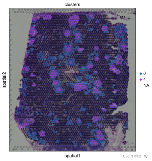
sc.pl.spatial(adata, img_key="hires", color="clusters", size=1.5)

Belonging to the same cluster in the gene expression space spots It usually appears in the spatial dimension at the same time . for example , Belong to cluster 4 Points of are usually classified as clusters 0 Surrounded by points .

We can zoom in on a particular region of interest , To reach a particular conclusion . Besides , By changing spot Of alpha value , We can better learn from H&E Potential tissue morphology seen in the image .

sc.pl.spatial(adata, img_key="hires", color="clusters", groups=["0", "4"], alpha=0.5, size=1.3)

Clustered marker gene

Let's examine the cluster further 4. We calculate the marker genes and draw a heat map , The figure shows the front... In the cluster 10 Expression levels of marker genes .

sc.tl.rank_genes_groups(adata, "clusters", method="t-test")
sc.pl.rank_genes_groups_heatmap(adata, groups="4", n_genes=10, groupby="clusters")

""" ranking genes finished: added to `.uns['rank_genes_groups']` 'names', sorted np.recarray to be indexed by group ids 'scores', sorted np.recarray to be indexed by group ids 'logfoldchanges', sorted np.recarray to be indexed by group ids 'pvals', sorted np.recarray to be indexed by group ids 'pvals_adj', sorted np.recarray to be indexed by group ids (0:00:02) WARNING: dendrogram data not found (using key=dendrogram_clusters). Running `sc.tl.dendrogram` with default parameters. For fine tuning it is recommended to run `sc.tl.dendrogram` independently. using 'X_pca' with n_pcs = 50 Storing dendrogram info using `.uns['dendrogram_clusters']` WARNING: Groups are not reordered because the `groupby` categories and the `var_group_labels` are different. categories: 0, 1, 2, etc. var_group_labels: 4 """

We are interested in genes CR2 Analyze ：

sc.pl.spatial(adata, img_key="hires", color=["clusters", "CR2"])

Hypervariable genes of spatial data

Spatial transcriptomics enables researchers to study changes in gene expression trends in space , So as to determine the spatial pattern of gene expression . So , We use SpatialDE, This is a statistical framework based on Gaussian process , Variable genes designed to identify spatial transcriptome ：

pip install spatialde

---

lately , Other tools for identifying spatially variant genes have also been proposed , for example ：SPARK,trendsceek,HMRF

---

First , We will standardize counts and coordinates Convert to pandas dataframe, This is the input spatialDE The required ：

import SpatialDE

%%time
counts = pd.DataFrame(adata.X.todense(), columns=adata.var_names, index=adata.obs_names)
coord = pd.DataFrame(adata.obsm['spatial'], columns=['x_coord', 'y_coord'], index=adata.obs_names)

""" CPU times: total: 93.8 ms Wall time: 94.7 ms """

see counts：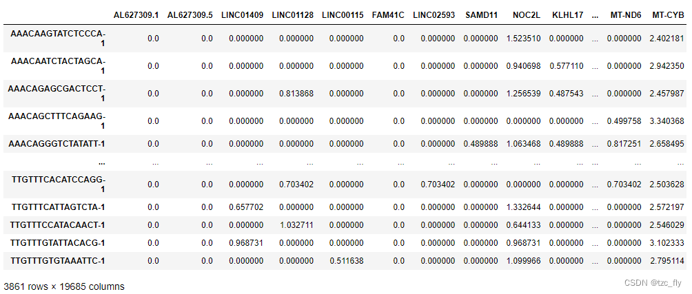

see coord：

function SpatialDE It takes quite a long time （ This example is close to 2 Hours ）.

results = SpatialDE.run(coord, counts)

results The variable genes calculated based on the spatial transcriptome data will be saved in .

MERFISH Example

If we use based on FISH Technology to generate spatial data , Just read cordinate Table and assign it to adata.obsm that will do .

Let's look at Xia wait forsomeone 2019 The example of .

First , We need to download coordinates and counts data ：

import urllib.request

url_coord = "https://www.pnas.org/highwire/filestream/887973/field_highwire_adjunct_files/15/pnas.1912459116.sd15.xlsx"
filename_coord = "pnas.1912459116.sd15.xlsx"
urllib.request.urlretrieve(url_coord, filename_coord)

url_counts = "https://www.pnas.org/highwire/filestream/887973/field_highwire_adjunct_files/12/pnas.1912459116.sd12.csv"
filename_counts = "pnas.1912459116.sd12.csv"
urllib.request.urlretrieve(url_counts, filename_counts)

---

If you can't access the above link , You can manually go to github download ：spatial datasets, This is the collation of a spatial transcription data set .

---

And then it reads adata：

coordinates = pd.read_excel("./pnas.1912459116.sd15.xlsx", index_col=0)
counts = sc.read_csv("./pnas.1912459116.sd12.csv").transpose()

adata_merfish = counts[coordinates.index, :]
adata_merfish.obsm["spatial"] = coordinates.to_numpy()

adata_merfish
""" AnnData object with n_obs × n_vars = 645 × 12903 obsm: 'spatial' """

We will perform standard preprocessing and dimensionality reduction ：

sc.pp.normalize_per_cell(adata_merfish, counts_per_cell_after=1e6)
sc.pp.log1p(adata_merfish)
sc.pp.pca(adata_merfish, n_comps=15)
sc.pp.neighbors(adata_merfish)
sc.tl.umap(adata_merfish)
sc.tl.leiden(adata_merfish, key_added="clusters", resolution=0.5)

""" normalizing by total count per cell finished (0:00:00): normalized adata.X and added 'n_counts', counts per cell before normalization (adata.obs) computing PCA with n_comps=15 finished (0:00:00) computing neighbors using 'X_pca' with n_pcs = 15 finished: added to `.uns['neighbors']` `.obsp['distances']`, distances for each pair of neighbors `.obsp['connectivities']`, weighted adjacency matrix (0:00:05) computing UMAP finished: added 'X_umap', UMAP coordinates (adata.obsm) (0:00:01) running Leiden clustering finished: found 7 clusters and added 'clusters', the cluster labels (adata.obs, categorical) (0:00:00) """

adata_merfish
""" AnnData object with n_obs × n_vars = 645 × 12903 obs: 'n_counts', 'clusters' uns: 'log1p', 'pca', 'neighbors', 'umap', 'leiden' obsm: 'spatial', 'X_pca', 'X_umap' varm: 'PCs' obsp: 'distances', 'connectivities' """

We can do it in UMAP Space and spatial Visualize in coordinates Leiden Resulting cluster .

sc.pl.umap(adata_merfish, color="clusters")
sc.pl.embedding(adata_merfish, basis="spatial", color="clusters")