当前位置:网站首页>Hands on deep learning (42) -- bi-directional recurrent neural network (BI RNN)
Hands on deep learning (42) -- bi-directional recurrent neural network (BI RNN)
2022-07-04 09:41:00 【Stay a little star】
List of articles
Two way recurrent neural network
In sequence learning , Our previously assumed goal is : up to now , Model the next output with a given observation . for example , In the context of time series or language models . Although this is a typical case , But this is not the only situation we may encounter . To illustrate the point , Consider the following three tasks for filling in the blanks in text sequences :
- I
___( happy 、 I'm hungry 、 very good …). - I
___I'm hungry ( very 、 commonly 、 already …). - I
___I'm hungry , I can eat half a pig ( very ).
According to the amount of information available , We can fill in the blanks with different words , Such as “ I'm very glad to ”(“happy”)、“ No ”(“not”) and “ very ”(“very”). Obviously , End of phrase ( If any ) It conveys an important message , And this information is about choosing which word to fill in the blank , Therefore, sequence models that cannot take advantage of this will perform poorly in related tasks . for example , If you want to do a good job in named entity recognition ( for example , distinguish “Green” refer to “ Mr. Green ” It's still green ), The importance of context ranges of different lengths is the same . In order to get some inspiration to solve the problem , Let's detour to the probability graph model first .
- It depends on the context of the past and the future , You can fill in very different words
- So far, RNN Just look at the past
- When filling in the blank , We can see the future
One 、 Dynamic programming in hidden Markov models
This section is used to illustrate the problem of dynamic programming , Specific technical details are not important for understanding the deep learning model , But they help people think about why they should use deep learning , And why choose a specific structure .( I can't understand the series when I look at it , It is recommended to skip if you don't understand , It doesn't affect reading , But it's also good to supplement probability theory )
If we want to solve this problem with probability graph model , You can design an implicit variable model , As shown in the figure below . At any time step t t t, Suppose there is an implicit variable h t h_t ht, Passing probability P ( x t ∣ h t ) P(x_t \mid h_t) P(xt∣ht) Control the emission we observe x t x_t xt. Besides , Any transfer h t → h t + 1 h_t \to h_{t+1} ht→ht+1 It is caused by some state transition probability P ( h t + 1 ∣ h t ) P(h_{t+1} \mid h_{t}) P(ht+1∣ht) give . This probability graph model is a hidden Markov model (hidden Markov model,HMM), As shown in the figure .

therefore , For having T T T A sequence of observations , We have the following joint probability distribution in the observed state and hidden state :
P ( x 1 , … , x T , h 1 , … , h T ) = ∏ t = 1 T P ( h t ∣ h t − 1 ) P ( x t ∣ h t ) , where P ( h 1 ∣ h 0 ) = P ( h 1 ) . P(x_1, \ldots, x_T, h_1, \ldots, h_T) = \prod_{t=1}^T P(h_t \mid h_{t-1}) P(x_t \mid h_t), \text{ where } P(h_1 \mid h_0) = P(h_1). P(x1,…,xT,h1,…,hT)=t=1∏TP(ht∣ht−1)P(xt∣ht), where P(h1∣h0)=P(h1).
Now suppose we observe all x i x_i xi, except x j x_j xj( Congratulations on entering the cloze screen ), And our goal is to calculate P ( x j ∣ x − j ) P(x_j \mid x_{-j}) P(xj∣x−j), among x − j = ( x 1 , … , x j − 1 , x j + 1 , … , x T ) x_{-j} = (x_1, \ldots, x_{j-1}, x_{j+1}, \ldots, x_{T}) x−j=(x1,…,xj−1,xj+1,…,xT). because P ( x j ∣ x − j ) P(x_j \mid x_{-j}) P(xj∣x−j) There are no hidden variables in , So let's consider h 1 , … , h T h_1, \ldots, h_T h1,…,hT All possible combinations formed by the choice of are summed . If anything h i h_i hi Acceptable k k k Different values ( A finite number of States ), This means that we need to know k T k^T kT Sum items , This task is impossible ! Fortunately, , There is an elegant solution —— Dynamic programming (dynamic programming).
Understand how it works , Consider for implicit variables h 1 , … , h T h_1, \ldots, h_T h1,…,hT Sum in sequence . We can draw :
P ( x 1 , … , x T ) = ∑ h 1 , … , h T P ( x 1 , … , x T , h 1 , … , h T ) = ∑ h 1 , … , h T ∏ t = 1 T P ( h t ∣ h t − 1 ) P ( x t ∣ h t ) = ∑ h 2 , … , h T [ ∑ h 1 P ( h 1 ) P ( x 1 ∣ h 1 ) P ( h 2 ∣ h 1 ) ] ⏟ π 2 ( h 2 ) = d e f P ( x 2 ∣ h 2 ) ∏ t = 3 T P ( h t ∣ h t − 1 ) P ( x t ∣ h t ) = ∑ h 3 , … , h T [ ∑ h 2 π 2 ( h 2 ) P ( x 2 ∣ h 2 ) P ( h 3 ∣ h 2 ) ] ⏟ π 3 ( h 3 ) = d e f P ( x 3 ∣ h 3 ) ∏ t = 4 T P ( h t ∣ h t − 1 ) P ( x t ∣ h t ) = … = ∑ h T π T ( h T ) P ( x T ∣ h T ) . \begin{aligned} &P(x_1, \ldots, x_T) \\ =& \sum_{h_1, \ldots, h_T} P(x_1, \ldots, x_T, h_1, \ldots, h_T) \\ =& \sum_{h_1, \ldots, h_T} \prod_{t=1}^T P(h_t \mid h_{t-1}) P(x_t \mid h_t) \\ =& \sum_{h_2, \ldots, h_T} \underbrace{\left[\sum_{h_1} P(h_1) P(x_1 \mid h_1) P(h_2 \mid h_1)\right]}_{\pi_2(h_2) \stackrel{\mathrm{def}}{=}} P(x_2 \mid h_2) \prod_{t=3}^T P(h_t \mid h_{t-1}) P(x_t \mid h_t) \\ =& \sum_{h_3, \ldots, h_T} \underbrace{\left[\sum_{h_2} \pi_2(h_2) P(x_2 \mid h_2) P(h_3 \mid h_2)\right]}_{\pi_3(h_3)\stackrel{\mathrm{def}}{=}} P(x_3 \mid h_3) \prod_{t=4}^T P(h_t \mid h_{t-1}) P(x_t \mid h_t)\\ =& \dots \\ =& \sum_{h_T} \pi_T(h_T) P(x_T \mid h_T). \end{aligned} ======P(x1,…,xT)h1,…,hT∑P(x1,…,xT,h1,…,hT)h1,…,hT∑t=1∏TP(ht∣ht−1)P(xt∣ht)h2,…,hT∑π2(h2)=def[h1∑P(h1)P(x1∣h1)P(h2∣h1)]P(x2∣h2)t=3∏TP(ht∣ht−1)P(xt∣ht)h3,…,hT∑π3(h3)=def[h2∑π2(h2)P(x2∣h2)P(h3∣h2)]P(x3∣h3)t=4∏TP(ht∣ht−1)P(xt∣ht)…hT∑πT(hT)P(xT∣hT).
Usually , We will “ Forward recursion ”(forward recursion) Written as :
π t + 1 ( h t + 1 ) = ∑ h t π t ( h t ) P ( x t ∣ h t ) P ( h t + 1 ∣ h t ) . \pi_{t+1}(h_{t+1}) = \sum_{h_t} \pi_t(h_t) P(x_t \mid h_t) P(h_{t+1} \mid h_t). πt+1(ht+1)=ht∑πt(ht)P(xt∣ht)P(ht+1∣ht).
Recursion is initialized to π 1 ( h 1 ) = P ( h 1 ) \pi_1(h_1) = P(h_1) π1(h1)=P(h1). Symbol simplification , Or you could write it as π t + 1 = f ( π t , x t ) \pi_{t+1} = f(\pi_t, x_t) πt+1=f(πt,xt), among f f f Are some learnable functions . This looks like the updating equation in the hidden variable model we discussed in the cyclic neural network .
Same as forward recursion , We can also use backward recursion to sum the same set of hidden variables . This will get :
P ( x 1 , … , x T ) = ∑ h 1 , … , h T P ( x 1 , … , x T , h 1 , … , h T ) = ∑ h 1 , … , h T ∏ t = 1 T − 1 P ( h t ∣ h t − 1 ) P ( x t ∣ h t ) ⋅ P ( h T ∣ h T − 1 ) P ( x T ∣ h T ) = ∑ h 1 , … , h T − 1 ∏ t = 1 T − 1 P ( h t ∣ h t − 1 ) P ( x t ∣ h t ) ⋅ [ ∑ h T P ( h T ∣ h T − 1 ) P ( x T ∣ h T ) ] ⏟ ρ T − 1 ( h T − 1 ) = d e f = ∑ h 1 , … , h T − 2 ∏ t = 1 T − 2 P ( h t ∣ h t − 1 ) P ( x t ∣ h t ) ⋅ [ ∑ h T − 1 P ( h T − 1 ∣ h T − 2 ) P ( x T − 1 ∣ h T − 1 ) ρ T − 1 ( h T − 1 ) ] ⏟ ρ T − 2 ( h T − 2 ) = d e f = … = ∑ h 1 P ( h 1 ) P ( x 1 ∣ h 1 ) ρ 1 ( h 1 ) . \begin{aligned} & P(x_1, \ldots, x_T) \\ =& \sum_{h_1, \ldots, h_T} P(x_1, \ldots, x_T, h_1, \ldots, h_T) \\ =& \sum_{h_1, \ldots, h_T} \prod_{t=1}^{T-1} P(h_t \mid h_{t-1}) P(x_t \mid h_t) \cdot P(h_T \mid h_{T-1}) P(x_T \mid h_T) \\ =& \sum_{h_1, \ldots, h_{T-1}} \prod_{t=1}^{T-1} P(h_t \mid h_{t-1}) P(x_t \mid h_t) \cdot \underbrace{\left[\sum_{h_T} P(h_T \mid h_{T-1}) P(x_T \mid h_T)\right]}_{\rho_{T-1}(h_{T-1})\stackrel{\mathrm{def}}{=}} \\ =& \sum_{h_1, \ldots, h_{T-2}} \prod_{t=1}^{T-2} P(h_t \mid h_{t-1}) P(x_t \mid h_t) \cdot \underbrace{\left[\sum_{h_{T-1}} P(h_{T-1} \mid h_{T-2}) P(x_{T-1} \mid h_{T-1}) \rho_{T-1}(h_{T-1}) \right]}_{\rho_{T-2}(h_{T-2})\stackrel{\mathrm{def}}{=}} \\ =& \ldots \\ =& \sum_{h_1} P(h_1) P(x_1 \mid h_1)\rho_{1}(h_{1}). \end{aligned} ======P(x1,…,xT)h1,…,hT∑P(x1,…,xT,h1,…,hT)h1,…,hT∑t=1∏T−1P(ht∣ht−1)P(xt∣ht)⋅P(hT∣hT−1)P(xT∣hT)h1,…,hT−1∑t=1∏T−1P(ht∣ht−1)P(xt∣ht)⋅ρT−1(hT−1)=def[hT∑P(hT∣hT−1)P(xT∣hT)]h1,…,hT−2∑t=1∏T−2P(ht∣ht−1)P(xt∣ht)⋅ρT−2(hT−2)=def⎣⎡hT−1∑P(hT−1∣hT−2)P(xT−1∣hT−1)ρT−1(hT−1)⎦⎤…h1∑P(h1)P(x1∣h1)ρ1(h1).
therefore , We can “ Backward recursion ”(backward recursion) Written as :
ρ t − 1 ( h t − 1 ) = ∑ h t P ( h t ∣ h t − 1 ) P ( x t ∣ h t ) ρ t ( h t ) , \rho_{t-1}(h_{t-1})= \sum_{h_{t}} P(h_{t} \mid h_{t-1}) P(x_{t} \mid h_{t}) \rho_{t}(h_{t}), ρt−1(ht−1)=ht∑P(ht∣ht−1)P(xt∣ht)ρt(ht),
initialization ρ T ( h T ) = 1 \rho_T(h_T) = 1 ρT(hT)=1. Both forward and backward recursion allow us to T T T There are hidden variables in O ( k T ) \mathcal{O}(kT) O(kT)( Linear rather than exponential ) Within the time ( h 1 , … , h T ) (h_1, \ldots, h_T) (h1,…,hT) Sum all values of . This is one of the great benefits of using graph model for probabilistic reasoning . It is also a general messaging Algorithm Aji.McEliece.2000 A very special example of . Combine forward and backward recursion , We can calculate
P ( x j ∣ x − j ) ∝ ∑ h j π j ( h j ) ρ j ( h j ) P ( x j ∣ h j ) . P(x_j \mid x_{-j}) \propto \sum_{h_j} \pi_j(h_j) \rho_j(h_j) P(x_j \mid h_j). P(xj∣x−j)∝hj∑πj(hj)ρj(hj)P(xj∣hj).
Notice the need for symbol simplification , Backward recursion can also be written as ρ t − 1 = g ( ρ t , x t ) \rho_{t-1} = g(\rho_t, x_t) ρt−1=g(ρt,xt), among g g g Is a function that can be learned . Again , This looks very much like a renewal equation , It's just not like the forward operation we see in the cyclic neural network , But backward calculation . in fact , Knowing when future data will be available is beneficial to hidden Markov models . Signal processing scientists divide whether they know about future observations into interpolation and extrapolation . For more details , see also Doucet.De Freitas.Gordon.2001.
Two 、 Two way model
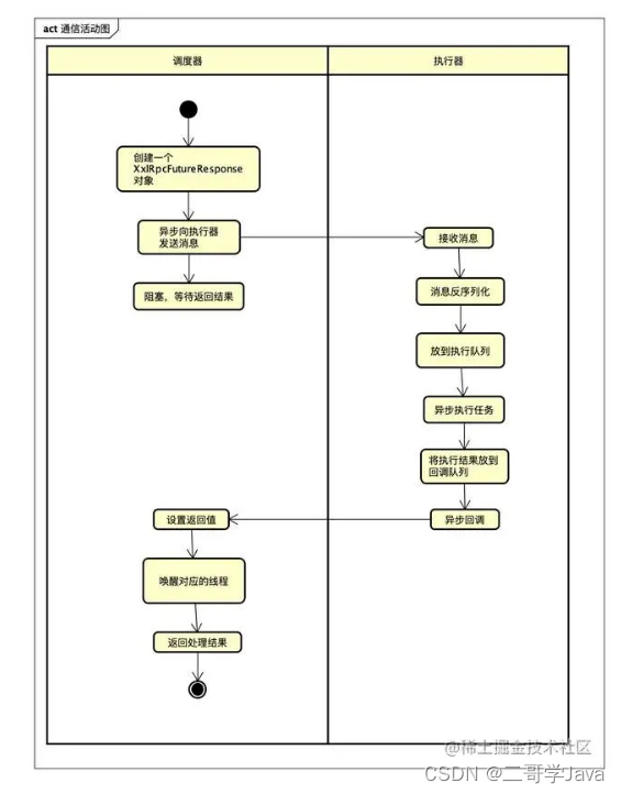
If we want to have a mechanism in recurrent neural networks , So that it can provide forward-looking ability similar to hidden Markov model , We need to modify the design of recurrent neural network . Fortunately, , This is conceptually easy , Just add a recurrent neural network that starts from the last mark and runs from back to front , Instead of just one recurrent neural network running from the first marker in forward mode .
Two way recurrent neural network (bidirectional RNNs) Added a hidden layer of reverse passing information , In order to deal with this kind of information more flexibly . The following figure describes the structure of a bidirectional recurrent neural network with a single hidden layer .

in fact , This is not much different from the forward and backward recursion of dynamic programming in hidden Markov models . The main difference is , The equations in hidden Markov models have specific statistical significance . There is no such easy explanation for bi-directional Recurrent Neural Networks , We can only regard them as general 、 Learnable functions . This transformation embodies the design principles of modern deep network : First, we use the function dependency type of classical statistical model , Then parameterize it into a general form .
2.1 Definition
Bidirectional recurrent neural network is composed of :Schuster.Paliwal.1997 Proposed , For a detailed discussion of various structures, see :Graves.Schmidhuber.2005. Let's take a look at the details of such a network .
For any time step t t t, Given a small batch of input data X t ∈ R n × d \mathbf{X}_t \in \mathbb{R}^{n \times d} Xt∈Rn×d( Sample size : n n n, The number of inputs in each example : d d d), And make the hidden layer activation function ϕ \phi ϕ. In a two-way structure , We set the forward and reverse hidden states of the time step as H → t ∈ R n × h \overrightarrow{\mathbf{H}}_t \in \mathbb{R}^{n \times h} Ht∈Rn×h and H ← t ∈ R n × h \overleftarrow{\mathbf{H}}_t \in \mathbb{R}^{n \times h} Ht∈Rn×h, among h h h Is the number of hidden units . The update of forward and reverse hidden status is as follows :
H → t = ϕ ( X t W x h ( f ) + H → t − 1 W h h ( f ) + b h ( f ) ) , H ← t = ϕ ( X t W x h ( b ) + H ← t + 1 W h h ( b ) + b h ( b ) ) , \begin{aligned} \overrightarrow{\mathbf{H}}_t &= \phi(\mathbf{X}_t \mathbf{W}_{xh}^{(f)} + \overrightarrow{\mathbf{H}}_{t-1} \mathbf{W}_{hh}^{(f)} + \mathbf{b}_h^{(f)}),\\ \overleftarrow{\mathbf{H}}_t &= \phi(\mathbf{X}_t \mathbf{W}_{xh}^{(b)} + \overleftarrow{\mathbf{H}}_{t+1} \mathbf{W}_{hh}^{(b)} + \mathbf{b}_h^{(b)}), \end{aligned} HtHt=ϕ(XtWxh(f)+Ht−1Whh(f)+bh(f)),=ϕ(XtWxh(b)+Ht+1Whh(b)+bh(b)),
among , The weight W x h ( f ) ∈ R d × h , W h h ( f ) ∈ R h × h , W x h ( b ) ∈ R d × h , W h h ( b ) ∈ R h × h \mathbf{W}_{xh}^{(f)} \in \mathbb{R}^{d \times h}, \mathbf{W}_{hh}^{(f)} \in \mathbb{R}^{h \times h}, \mathbf{W}_{xh}^{(b)} \in \mathbb{R}^{d \times h}, \mathbf{W}_{hh}^{(b)} \in \mathbb{R}^{h \times h} Wxh(f)∈Rd×h,Whh(f)∈Rh×h,Wxh(b)∈Rd×h,Whh(b)∈Rh×h And offset b h ( f ) ∈ R 1 × h , b h ( b ) ∈ R 1 × h \mathbf{b}_h^{(f)} \in \mathbb{R}^{1 \times h}, \mathbf{b}_h^{(b)} \in \mathbb{R}^{1 \times h} bh(f)∈R1×h,bh(b)∈R1×h All model parameters .
Next , Hide forward H → t \overrightarrow{\mathbf{H}}_t Ht And reverse hidden state H ← t \overleftarrow{\mathbf{H}}_t Ht Straight up , Get the hidden state that needs to be sent to the output layer H t ∈ R n × 2 h \mathbf{H}_t \in \mathbb{R}^{n \times 2h} Ht∈Rn×2h. In a deep bidirectional recurrent neural network with multiple hidden layers , This information is passed as input to the next two-way layer . Last , The output calculated by the output layer is O t ∈ R n × q \mathbf{O}_t \in \mathbb{R}^{n \times q} Ot∈Rn×q( q q q Is the number of output units ):
O t = H t W h q + b q . \mathbf{O}_t = \mathbf{H}_t \mathbf{W}_{hq} + \mathbf{b}_q. Ot=HtWhq+bq.
here , Weight matrices W h q ∈ R 2 h × q \mathbf{W}_{hq} \in \mathbb{R}^{2h \times q} Whq∈R2h×q And offset b q ∈ R 1 × q \mathbf{b}_q \in \mathbb{R}^{1 \times q} bq∈R1×q Is the model parameter of the output layer . in fact , These two directions can have different numbers of hidden units .
Forward and reverse weight yes concate Together , Not adding or other operations
2.2 The calculation cost of the model and Its Application
A key characteristic of bi-directional recurrent neural networks is , Use the information from both ends of the sequence to estimate the output . in other words , We use information from past and future observations to predict current observations . But in the case of predicting the next marker , Such behavior is not what we want . Because when predicting the next marker , After all, we can't know what the next mark is . therefore , If we are naive to predict based on bidirectional recurrent neural network , Will not get good accuracy : Because during training , We can use past and future data to estimate the present , During the test , We only have data from the past , So the accuracy will be very poor . below , We will explain this in the experiment .
Another serious problem is , The computing speed of bidirectional recurrent neural network is very slow . The main reason is that the forward propagation of the network requires forward and backward recursion in the two-way layer , And the back propagation of the network also depends on the result of forward propagation . therefore , The gradient solution will have a very long dependency chain .
The use of two-way layers is very rare in practice , And it is only used in some occasions . for example , Fill in the missing words 、 marker annotations ( for example , be used for Named entity recognition ) And encoding the sequence as a step in the sequence processing workflow ( for example , be used for Machine translation ).
3、 ... and 、 Wrong application of bidirectional recurrent neural network
as everyone knows , It is true that bi-directional recurrent neural networks use past and future data , And if we ignore those suggestions based on facts , And apply it to the language model , Then we can also get an acceptable degree of confusion . For all that , As shown in the following experiment , The ability of this model to predict future markers also has serious defects . Although the degree of confusion is reasonable , But after many iterations, the model can only generate garbled code . We use the following code as a warning , In case they are used in the wrong environment .( Complete the cloze , Not inferential , Actually, it's quite understandable , It's because we know and use the future information during training , In practical reasoning, future information is unknown )
''' warning !!! Here is a wrong example Used to describe two-way LSTM Cannot be used to predict ! The result of its confusion is really good , But it's almost impossible to predict the future '''
import torch
from torch import nn
from d2l import torch as d2l
# Load data
batch_size,num_steps,device = 32,25,d2l.try_gpu()
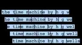
train_iter,vocab = d2l.load_data_time_machine(batch_size,num_steps)
# By setting ‘bidirective=True’ Define bidirectional LSTM
vocab_size, num_hiddens, num_layers = len(vocab), 256, 2
num_inputs = vocab_size
lstm_layer = nn.LSTM(num_inputs, num_hiddens, num_layers, bidirectional=True)
model = d2l.RNNModel(lstm_layer, len(vocab))
model = model.to(device)
# Training models
num_epochs, lr = 500, 1
d2l.train_ch8(model, train_iter, vocab, lr, num_epochs, device)
perplexity 1.1, 77803.5 tokens/sec on cuda:0
time travellerererererererererererererererererererererererererer
travellerererererererererererererererererererererererererer

边栏推荐
- Analysis report on the development status and investment planning of China's modular power supply industry Ⓠ 2022 ~ 2028
- 2022-2028 global seeder industry research and trend analysis report
- Some points needing attention in PMP learning
- Reload CUDA and cudnn (for tensorflow and pytorch) [personal sorting summary]
- 2022-2028 global elastic strain sensor industry research and trend analysis report
- How web pages interact with applets
- C language pointer classic interview question - the first bullet
- Investment analysis and future production and marketing demand forecast report of China's paper industry Ⓥ 2022 ~ 2028
- Kotlin:集合使用
- xxl-job惊艳的设计,怎能叫人不爱
猜你喜欢

2022-2028 global elastic strain sensor industry research and trend analysis report
2022-2028 global gasket plate heat exchanger industry research and trend analysis report

PHP book borrowing management system, with complete functions, supports user foreground management and background management, and supports the latest version of PHP 7 x. Database mysql
xxl-job惊艳的设计,怎能叫人不爱

How does idea withdraw code from remote push

At the age of 30, I changed to Hongmeng with a high salary because I did these three things
C language pointer classic interview question - the first bullet
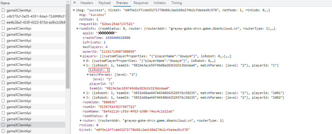
华为联机对战如何提升玩家匹配成功几率
Hands on deep learning (36) -- language model and data set
2022-2028 global seeder industry research and trend analysis report
随机推荐
Global and Chinese market of sampler 2022-2028: Research Report on technology, participants, trends, market size and share
Upgrading Xcode 12 caused Carthage to build cartfile containing only rxswift to fail
How to batch change file extensions in win10
2022-2028 global small batch batch batch furnace industry research and trend analysis report
技术管理进阶——如何设计并跟进不同层级同学的绩效
Hands on deep learning (33) -- style transfer
mmclassification 标注文件生成
Lauchpad x | MODE
Fabric of kubernetes CNI plug-in
Global and Chinese markets of thrombography hemostasis analyzer (TEG) 2022-2028: Research Report on technology, participants, trends, market size and share
Latex download installation record
H5 audio tag custom style modification and adding playback control events
2022-2028 global tensile strain sensor industry research and trend analysis report
pcl::fromROSMsg报警告Failed to find match for field ‘intensity‘.
C # use gdi+ to add text with center rotation (arbitrary angle)
查看CSDN个人资源下载明细
Investment analysis and prospect prediction report of global and Chinese high purity tin oxide Market Ⓞ 2022 ~ 2027
How do microservices aggregate API documents? This wave of show~
At the age of 30, I changed to Hongmeng with a high salary because I did these three things
HMS core helps baby bus show high-quality children's digital content to global developers