当前位置:网站首页>Combat readiness mathematical modeling 31 data interpolation and curve fitting 3
Combat readiness mathematical modeling 31 data interpolation and curve fitting 3
2022-06-26 14:28:00 【nuist__ NJUPT】
Catalog
One 、 Classic cases of data interpolation
Two 、 Curve fitting classic case
One 、 Classic cases of data interpolation
The following is pool 1 1,3,5...15 Various indicators of the week , Interpolate the indicators in the pool , And all the images drawn after interpolation are displayed on one graph .
More data , It is troublesome to select each row for interpolation , Circular interpolation possible , then subplot Function to draw multiple graphs , Of course , For one-dimensional interpolation , We prefer cubic spline interpolation .

Concrete MATLAB The code is as follows :
clear; clc
load('Z.mat')
x = Z(1,:) ; % Get a row vector , Weeks
[n,m] = size(Z) ; % Get the number of rows and columns of the original data
% Each picture y The label of the shaft
ylab={' Weeks ',' rotifer ',' Dissolved oxygen ','COD',' The water temperature ','PH value ',' Salinity ',' transparency ',' Total alkalinity ',' Chloride ion ',' transparency ',' Biomass '};
P = zeros(11,15) ;

for i = 2 : n % From 2 Row start interpolation
    y = Z(i,:) ;
    new_x = 1:15 ;
    p1 = interp1(x,y,new_x,'spline') ; % Cubic spline interpolation
    subplot(4,3,i-1) ;
    plot(x,y,'ro',new_x,p1,'-');
    axis([0 15,-inf,inf]) ;
    xlabel(' Weeks ') ;
    ylabel(ylab(i)) ;
    P(i-1,:) = p1 ;
end
legend(' Raw data ',' Cubic spline interpolation data ','Location','SouthEast'); % legend
disp(P) ;
The drawing is as follows :

Two 、 Curve fitting classic case
1- Polynomial fitting
Let's look at a simple example , The following data are fitted by polynomial , Of course, it can be directly fitted and solved , That is to solve the linear regression equation of one variable , It can also be solved by the least square method , In addition to drawing the fitting curve , The goodness of fit is also calculated .

MATLAB The code is as follows :
Method 1, Direct polynomial fitting
clear; clc
load('nihe.mat');
%plot(x,y,'o') ;
xlabel('x Value ') ;
ylabel('y Value ') ;
n = size(x,1) ; % Number of sample points
x = x' ;
y = y' ;
xp = 2.7 : 0.1 : 6.9 ;
p = polyfit(x,y,1) ;
yp = polyval(p,xp);
plot(x,y,'o',xp,yp) ;
legend(' Sample data ',' Fit function ','location','SouthEast') ;
Method 2, Least squares parameter estimation , Then draw according to the expression , The goodness of fit is calculated here .
clear; clc
load('nihe.mat');
plot(x,y,'o') ;
xlabel('x Value ') ;
ylabel('y Value ') ;
n = size(x,1) ; % Number of sample points
% Least square method for parameter estimation
k = (n*sum(x.*y)-sum(x)*sum(y))/(n*sum(x.*x)-sum(x)*sum(x)) ;
b = (sum(x.*x)*sum(y)-sum(x)*sum(x.*y))/(n*sum(x.*x)-sum(x)*sum(x)) ;
hold on ;
grid on ;
f = @(x) k*x + b ; % Anonymous functions
fplot(f,[1,7.5]) ;
legend(' Sample data ',' Fit function ','location','SouthEast') ;
y_hat = k * x + b ;
SSR = sum((y_hat-mean(y)).^2) ; % Sum of regression squares
SSE = sum((y_hat-y).^2) ; % The sum of the squares of the errors
SST = sum((y-mean(y)).^2) ; % Total sum of squares
disp(' Goodness of fit values are as follows :') ;
R_2= SSR / SST ;
disp(R_2) ;
The explanation of goodness of fit is as follows : The goodness of fit is closer to 1, The smaller the sum of squared errors , The better the fitting effect is .

The drawing is as follows :

2- Nonlinear fitting
Let's take a look at the envious population forecast , The nonlinear fitting function can be used directly , You can also use the fitting toolbox cftool

MATLAB The code is as follows , Here, nonlinear fitting is performed directly , Anonymous functions are required .
clear; clc
x = 1790:10:2000;
y = [3.9,5.3,7.2,9.6,12.9,17.1,23.2,31.4,38.6,50.2,62.9,76.0,92.0,106.5,123.2,131.7,150.7,179.3,204.0,226.5,251.4,281.4];
plot(x,y,'o')
y1 = @(b,t) b(1) ./ (1 + (b(1) / 3.9 - 1)*exp(-b(2)*(t-1790))); % Anonymous functions
b0 = [100 0.1] ; % The selection of initial value is very important
a = nlinfit(x,y,y1,b0)  ; % Coefficient after nonlinear fitting
xp = 1790 : 10 : 2030 ;
yp = y1(a,xp) ; % Substitute coefficients and values into the expression for evaluation
hold on ;
plot(xp, yp, '-') ;
legend(' Original scatter ',' Fit the curve ') ;
The drawing is as follows :

边栏推荐
- Sword finger offer 09.30 Stack
- Assert and constd13
- 【async/await】--异步编程最终解决方案
- Hard (magnetic) disk (I)
- When drawing with origin, capital letter C will appear in the upper left corner of the chart. The removal method is as follows:
- 9項規定6個嚴禁!教育部、應急管理部聯合印發《校外培訓機構消防安全管理九項規定》
- 数学建模经验分享:国赛美赛对比/选题参考/常用技巧
- Record: why is there no lightning 4 interface graphics card docking station and mobile hard disk?
- FreeFileSync 文件夹比较与同步软件
- Build your own PE manually from winpe of ADK
猜你喜欢

Wechat applet Registration Guide

Self created notes (unique in the whole network, continuously updated)

FreeFileSync 文件夹比较与同步软件

9项规定6个严禁!教育部、应急管理部联合印发《校外培训机构消防安全管理九项规定》

Matplotlib common operations

Setup instance of layout manager login interface
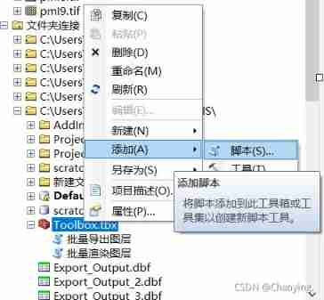
ArcGIS batch render layer script
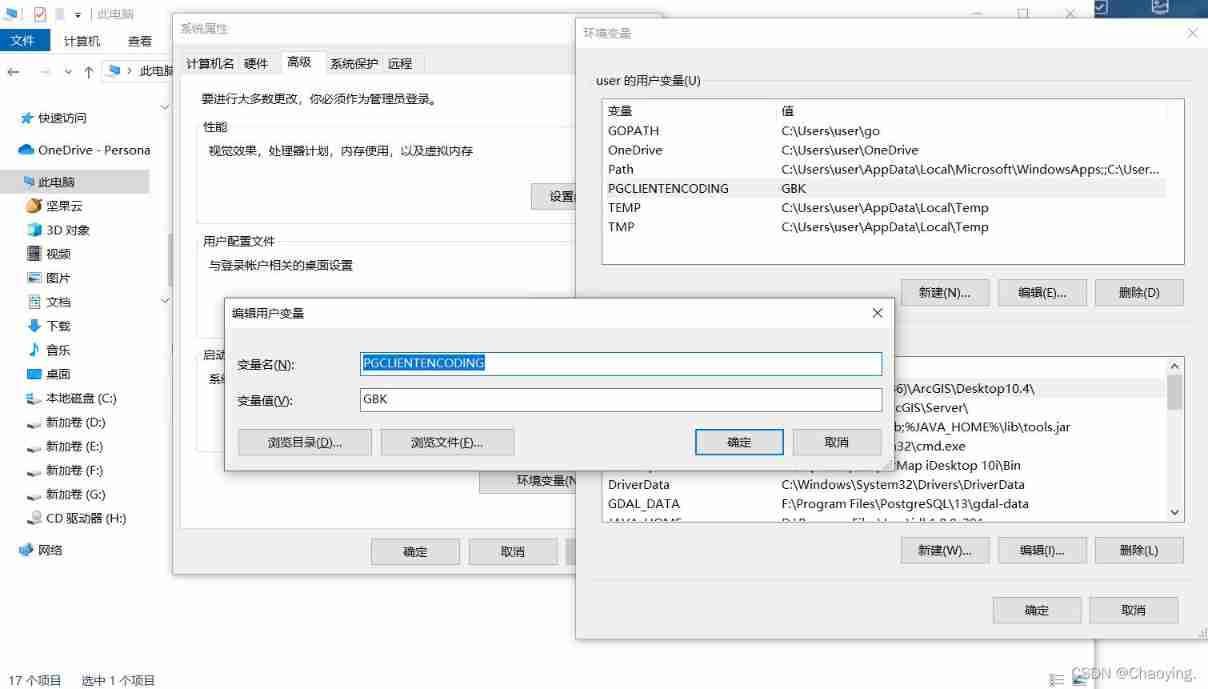
Chinese output of PostGIS console is garbled

Pycharm远程连接服务器来跑代码

ArcGIS cannot be opened and displays' because afcore cannot be found ' DLL, solution to 'unable to execute code'
随机推荐
Online bull Blogger
Installation tutorial about origin2019
PostGIS create spatial database
量化框架backtrader之一文读懂observer观测器
Bug STL string
Common operation and Principle Exploration of stream
'教练,我想打篮球!' —— 给做系统的同学们准备的 AI 学习系列小册
D - Face Produces Unhappiness
Hard (magnetic) disk (I)
Sword finger offer 05.58 Ⅱ string
Installation and uninstallation of MySQL software for windows
"Scoi2016" delicious problem solution
ArcGIS batch render layer script
2022年最新贵州建筑八大员(机械员)模拟考试题库及答案
Question bank and answers of the latest Guizhou construction eight (Mechanics) simulated examination in 2022
Memory considerations under bug memory management
oracle11g数据库导入导出方法教程[通俗易懂]
On insect classes and objects
ThreadLocal巨坑!内存泄露只是小儿科...
From Celsius to the three arrows: encrypting the domino of the ten billion giants, and drying up the epic liquidity