当前位置:网站首页>Seura 2测试代码总结
Seura 2测试代码总结
2022-06-29 03:27:00 【qq_45759229】
参考文献
https://www.jianshu.com/p/6b61dc92677c

https://davetang.org/muse/2017/08/01/getting-started-seurat/
运行代码
rm(list=ls())
setwd("/DATA2/zhangjingxiao/yxk/dataset/pancreas_Seurat2/")
suppressMessages(library(Seurat))
suppressMessages(library(ggplot2))
print(packageVersion("Seurat"))

library(Seurat)
### 构建Seurat对象
pancreas.data <- readRDS(file = "pancreas_expression_matrix.rds")
metadata <- readRDS(file = "pancreas_metadata.rds")
pancreas <- CreateSeuratObject(raw.data = pancreas.data, meta.data = metadata)

### 分离4种技术测序数据,构建独立对象
pancreas.list <- SplitObject(object = pancreas,attribute.1 = "tech")
celseq <- pancreas.list$celseq
celseq2 <- pancreas.list$celseq2
fluidigmc1 <- pancreas.list$fluidigmc1
smartseq2 <- pancreas.list$smartseq2

### QC and normalize, preprocessing
# for celseq data
celseq <- FilterCells(celseq, subset.names = "nGene", low.thresholds = 1750)
celseq <- NormalizeData(celseq)
celseq <- FindVariableGenes(celseq, do.plot = F, display.progress = F)
celseq <- ScaleData(celseq)
# for celseq2 data
celseq2 <- FilterCells(celseq2, subset.names = "nGene", low.thresholds = 2500)
celseq2 <- NormalizeData(celseq2)
celseq2 <- FindVariableGenes(celseq2, do.plot = F, display.progress = F)
celseq2 <- ScaleData(celseq2)
# for fluidigmc1 data, already filtered and no need to FilterCells again
fluidigmc1 <- NormalizeData(fluidigmc1)
fluidigmc1 <- FindVariableGenes(fluidigmc1, do.plot = F, display.progress = F)
fluidigmc1 <- ScaleData(fluidigmc1)
# for smartseq2 data
smartseq2 <- FilterCells(smartseq2, subset.names = "nGene", low.thresholds = 2500)
smartseq2 <- NormalizeData(smartseq2)
smartseq2 <- FindVariableGenes(smartseq2, do.plot = F, display.progress = F)
smartseq2 <- ScaleData(smartseq2)

### 对数据进行采样,每个数据集随机选取500个细胞进行下游分析,以减少内存消耗,缩短分析时间
celseq <- SetAllIdent(celseq, id = "tech")
celseq <- SubsetData(celseq, max.cells.per.ident = 500, random.seed = 1)
celseq2 <- SetAllIdent(celseq2, id = "tech")
celseq2 <- SubsetData(celseq2, max.cells.per.ident = 500, random.seed = 1)
fluidigmc1 <- SetAllIdent(fluidigmc1, id = "tech")
fluidigmc1 <- SubsetData(fluidigmc1, max.cells.per.ident = 500, random.seed = 1)
smartseq2 <- SetAllIdent(smartseq2, id = "tech")
smartseq2 <- SubsetData(smartseq2, max.cells.per.ident = 500, random.seed = 1)

# 将预处理好的数据存储备用
save(celseq, celseq2, fluidigmc1, smartseq2, file='splited.4.seurat.object.RData')

## 基本上是一样的,没有什么问题
#ggsave("vis_splatter.png",plot=p1+p2)

# Merge Seurat objects
gcdata <- MergeSeurat(celseq, celseq2, do.normalize=F)
gcdata <- MergeSeurat(gcdata, fluidigmc1, do.normalize=F)
gcdata <- MergeSeurat(gcdata, smartseq2, do.normalize=F)

# 查看不同4种技术之间在测得基因数量上的差异,如图1所示
VlnPlot(gcdata, "nGene", group.by = "tech")

# 对汇总后的数据进行矫正和归一化
gcdata <- NormalizeData(object = gcdata)
gcdata <- FindVariableGenes(gcdata, do.plot = F, display.progress = F)
gcdata <- ScaleData(gcdata, genes.use = gcdata@var.genes)
# PCA降维
gcdata <- RunPCA(gcdata, pc.genes = gcdata@var.genes,
pcs.compute = 30, do.print = TRUE, pcs.print = 5, genes.print = 5)
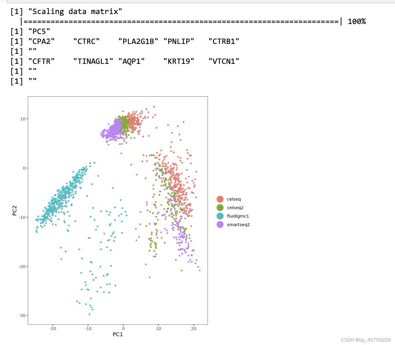
# 查看细胞在PCA前两个维度空间中的分布,观察有无批次效应,如图2所示
# 可以用看出细胞分布受批次效应影响较大,尤其是Fluidigm C1数据集与其他数据集存在明显偏离
DimPlot(gcdata, reduction.use = "pca", dim.1 = 1, dim.2 = 2, group.by = "tech")
# 聚类并进行tSNE降维
gcdata <- FindClusters(gcdata, reduction.type = "pca", dims.use = 1:20,
          print.output = F, save.SNN = T, force.recalc = T, random.seed = 100)
gcdata <- RunTSNE(gcdata, dims.use = 1:20, do.fast = T, reduction.use = "pca", perplexity = 30)
# 在tSNE降维空间查看细胞聚类结果与批次分布,如图3所示。
# 可看出细胞聚类结果受到批次效应影响较大,同一细胞群基本来自同一批次
p1 <- DimPlot(gcdata, reduction.use = "tsne", dim.1 = 1, dim.2 = 2, group.by = "res.0.8")
p2 <- DimPlot(gcdata, reduction.use = "tsne", dim.1 = 1, dim.2 = 2, group.by = "tech")
plot_grid(p1, p2)


# 根据Adjusted rand index(ARI)系数对批次效应进行评价
# ARI对当前聚类结果与4种技术标签进行比较,ARI值在-1到1之间
# ARI接近于1说明两种聚类标签具有很高的相似性
# ARI接近于0说明一种聚类标签相对于另一种为随机产生
# ARI小于0说明两种聚类标签相似性甚至低于随机水平(此处存疑)
# 具体计算过程见https://davetang.org/muse/2017/09/21/adjusted-rand-index/
# 自然,我们希望当前聚类结果与4种技术标签互相独立,ARI值应接近于0
# 结果结果显示ARI为0.3430069,说明当前聚类结果受到批次效应影响
ari <- dplyr::select(gcdata@meta.data, tech, res.0.8)
ari$tech <- plyr::mapvalues(ari$tech, from = c("celseq", "celseq2", "fluidigmc1", "smartseq2"), to = c(0, 1, 2, 3))
mclust::adjustedRandIndex(as.numeric(ari$tech), as.numeric(ari$res.0.8))

# 保存当前结果
save(gcdata, file = "gcdata.Rdata")

# 鉴定出至少在两个数据集中同时出现的高变异基因,使用这些基因进行CCA分析
ob.list <- list(celseq, celseq2, fluidigmc1, smartseq2)
genes.use <- c()
for (i in 1:length(ob.list)) {

    genes.use <- c(genes.use, head(rownames(ob.list[[i]]@hvg.info), 1000))
}
genes.use <- names(which(table(genes.use) > 1))
for (i in 1:length(ob.list)) {

    genes.use <- genes.use[genes.use %in% rownames(ob.list[[i]]@scale.data)]
}

# 使用上述程序鉴定到的高变异基因,对4个数据集进行CCA分析,并计算前15个CC维度
gcdata.CCA <- RunMultiCCA(ob.list, genes.use = genes.use, num.ccs = 15)

# 查看细胞在CCA前两个维度空间中的分布,观察有无批次效应,如图4所示
# 可以看出与图2相比,批次效应得到一定程度的缓解
DimPlot(gcdata.CCA, reduction.use = "cca", group.by = "tech", pt.size = 0.5)

# 查看在前几个CC维度上重要性较大的部分基因,这些基因的表达可能在细胞类别的区分上权重较大,如图5所示
DimHeatmap(object = gcdata.CCA, reduction.type = "cca", cells.use = 500, dim.use = 1:9, do.balanced = TRUE)

# 使用MetageneBicorPlot功能,选择下游分析使用的CC维度,如图6所示
# 可选择前10-12个CC维度进行下游分析
MetageneBicorPlot(gcdata.CCA, grouping.var = "tech", dims.eval = 1:15)

# 将4个数据集的CCA维度空间进行比对,产生新的降维空间cca.aligned
# 在新的空间对细胞进行聚类分析
# 使用AlignSubspace,同时声明分组变量与比对维度
gcdata.CCA <- AlignSubspace(gcdata.CCA, grouping.var = "tech", dims.align = 1:12)

# 查看比对之后的维度分数分布,如图7所示
VlnPlot(gcdata.CCA, features.plot = c("ACC1","ACC2"),, group.by = "tech")

# 与未比对之前的CC维度分数分布进行比较,如图8所示
# 图7、图8比较,可见经过CCA比对之后,细胞分布收到批次效应影响的程度更小
VlnPlot(gcdata.CCA, features.plot = c("CC1","CC2"),, group.by = "tech")

# 在比对后的ACC空间进行聚类分析与tSNE降维分析
gcdata.CCA <- FindClusters(gcdata.CCA, reduction.type = "cca.aligned", dims.use = 1:12,
              save.SNN = T, random.seed = 100)
gcdata.CCA <- RunTSNE(gcdata.CCA, reduction.use = "cca.aligned", dims.use = 1:12,
              do.fast = TRUE, seed.use = 1)

# 在tSNE降维空间查看细胞聚类结果与批次分布,如图9所示
# 与图3比较,可见批次效应得到很大程度的缓解,各个批次的细胞呈均匀分布
p1 <- DimPlot(gcdata.CCA, reduction.use = "tsne", dim.1 = 1, dim.2 = 2,
      group.by = "res.0.8", do.return = T)
p2 <- DimPlot(gcdata.CCA, reduction.use = "tsne", dim.1 = 1, dim.2 = 2,
      group.by = "tech", do.return = T)
plot_grid(p1, p2)

sessionInfo()
R version 4.0.3 (2020-10-10)
Platform: x86_64-conda-linux-gnu (64-bit)
Running under: Ubuntu 16.04.1 LTS

Matrix products: default
BLAS/LAPACK: /home/zhangjingxiao/.conda/envs/Seurat2/lib/libopenblasp-r0.3.20.so

locale:
 [1] LC_CTYPE=C.UTF-8    LC_NUMERIC=C        LC_TIME=C
 [4] LC_COLLATE=C        LC_MONETARY=C       LC_MESSAGES=C
 [7] LC_PAPER=C          LC_NAME=C           LC_ADDRESS=C
[10] LC_TELEPHONE=C      LC_MEASUREMENT=C    LC_IDENTIFICATION=C

attached base packages:
[1] stats     graphics  grDevices utils     datasets  methods   base

other attached packages:
[1] Seurat_2.3.0  Matrix_1.4-1  cowplot_1.1.1 ggplot2_3.3.6

loaded via a namespace (and not attached):
  [1] uuid_1.1-0           snow_0.4-4           backports_1.4.1
  [4] Hmisc_4.7-0          VGAM_1.1-6           sn_2.0.2
  [7] plyr_1.8.7           igraph_1.3.2         repr_1.1.4
 [10] splines_4.0.3        listenv_0.8.0        TH.data_1.1-1
 [13] digest_0.6.29        foreach_1.5.2        htmltools_0.5.2
 [16] lars_1.3             gdata_2.18.0.1       fansi_1.0.3
 [19] magrittr_2.0.3       checkmate_2.1.0      cluster_2.1.3
 [22] mixtools_1.2.0       ROCR_1.0-11          recipes_0.2.0
 [25] globals_0.15.1       gower_1.0.0          R.utils_2.11.0
 [28] sandwich_3.0-2       hardhat_1.1.0        jpeg_0.1-9
 [31] colorspace_2.0-3     rbibutils_2.2.8      xfun_0.31
 [34] dplyr_1.0.9          crayon_1.5.1         jsonlite_1.8.0
 [37] survival_3.3-1       zoo_1.8-10           iterators_1.0.14
 [40] ape_5.6-2            glue_1.6.2           gtable_0.3.0
 [43] ipred_0.9-13         kernlab_0.9-31       future.apply_1.9.0
 [46] prabclus_2.3-2       BiocGenerics_0.36.1  DEoptimR_1.0-11
 [49] scales_1.2.0         mvtnorm_1.1-3        Rcpp_1.0.8.3
 [52] metap_1.4            dtw_1.22-3           plotrix_3.8-2
 [55] htmlTable_2.4.0      tclust_1.5-1         foreign_0.8-82
 [58] proxy_0.4-27         mclust_5.4.10        SDMTools_1.1-221.1
 [61] Formula_1.2-4        tsne_0.1-3.1         stats4_4.0.3
 [64] lava_1.6.10          prodlim_2019.11.13   htmlwidgets_1.5.4
 [67] gplots_3.1.3         FNN_1.1.3.1          RColorBrewer_1.1-3
 [70] fpc_2.2-9            TFisher_0.2.0        modeltools_0.2-23
 [73] ellipsis_0.3.2       ica_1.0-2            farver_2.1.0
 [76] pkgconfig_2.0.3      R.methodsS3_1.8.2    flexmix_2.3-18
 [79] nnet_7.3-17          utf8_1.2.2           caret_6.0-92
 [82] labeling_0.4.2       tidyselect_1.1.2     rlang_1.0.2
 [85] reshape2_1.4.4       munsell_0.5.0        tools_4.0.3
 [88] cli_3.3.0            generics_0.1.2       ranger_0.14.1
 [91] ggridges_0.5.3       mathjaxr_1.6-0       evaluate_0.15
 [94] stringr_1.4.0        fastmap_1.1.0        ModelMetrics_1.2.2.2
 [97] knitr_1.39           fitdistrplus_1.1-8   robustbase_0.95-0
[100] caTools_1.18.2       purrr_0.3.4          RANN_2.6.1
[103] pbapply_1.5-0        future_1.26.1        nlme_3.1-158
[106] R.oo_1.25.0          compiler_4.0.3       rstudioapi_0.13
[109] png_0.1-7            tibble_3.1.7         stringi_1.7.6
[112] lattice_0.20-45      IRdisplay_1.1        multtest_2.6.0
[115] vctrs_0.4.1          mutoss_0.1-12        diffusionMap_1.2.0
[118] pillar_1.7.0         lifecycle_1.0.1      lmtest_0.9-40
[121] Rdpack_2.3.1         irlba_2.3.5          bitops_1.0-7
[124] data.table_1.14.2    R6_2.5.1             latticeExtra_0.6-29
[127] KernSmooth_2.23-20   gridExtra_2.3        parallelly_1.32.0
[130] codetools_0.2-18     gtools_3.9.2.2       MASS_7.3-57
[133] withr_2.5.0          mnormt_2.1.0         multcomp_1.4-19
[136] mgcv_1.8-40          diptest_0.76-0       parallel_4.0.3
[139] doSNOW_1.0.20        grid_4.0.3           rpart_4.1.16
[142] timeDate_3043.102    IRkernel_1.3         tidyr_1.2.0
[145] class_7.3-20         segmented_1.6-0      Rtsne_0.16
[148] pbdZMQ_0.3-7         pROC_1.18.0          numDeriv_2016.8-1.1
[151] scatterplot3d_0.3-41 Biobase_2.50.0       lubridate_1.8.0
[154] base64enc_0.1-3
边栏推荐
- 【雲原生】這麼火,你不來了解下?
- Gartner“客户之声”最高分,用户体验成中国数据库一大突破口
- Farrowtech's wireless sensor adopts the nanobeacon Bluetooth beacon technology of orange group Microelectronics
- Etcd tutorial - Chapter 6 etcd core API V3
- [tcapulusdb knowledge base] Introduction to tcapulusdb data import
- 迅为i.MX8M开发板yocto系统使用Gstarwmr视频转换
- 恢复二叉搜索树[根据题意模拟->发现问题->分析问题->见招拆招]
- 【TcaplusDB知识库】TcaplusDB-tcaplusadmin工具介绍
- MATALB signal processing - signal transformation (7)
- Mobaihe box, ZTE box, Migu box, Huawei box, Huawei Yuehe box, Fiberhome box, Skyworth box, Tianyi box and other operators' box firmware collection and sharing
猜你喜欢
![Jerry's watch obtains alarm mode settings [chapter]](/img/43/987d864ec6038b10138ce50bcbdf12.jpg)
Jerry's watch obtains alarm mode settings [chapter]

88.(cesium篇)cesium聚合图
 [email protected]"/>
无法定位程序输入点 [email protected]

分享 60 个神级 VS Code 插件
![恢复二叉搜索树[根据题意模拟->发现问题->分析问题->见招拆招]](/img/06/cc3c512e69455416fe81943bebacca.png)
恢复二叉搜索树[根据题意模拟->发现问题->分析问题->见招拆招]

2D人体姿态估计 - DeepPose
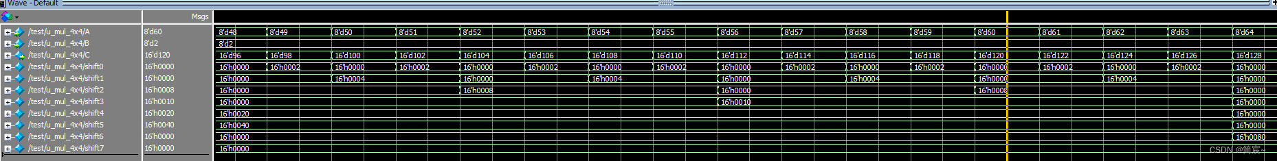
FPGA (VIII) RTL code IV (basic circuit design 1)
![相同的树[从部分到整体]](/img/2d/997b9cb9cd4f8ea8620f5a66fcf00a.png)
相同的树[从部分到整体]
![Movement state change of monitoring device of Jerry's watch [chapter]](/img/ff/cbc9e50a7d64e943f9f9924eadb184.jpg)
Movement state change of monitoring device of Jerry's watch [chapter]
![Jerry's watch pause [chapter]](/img/57/487ca3dd40e5a7bafdbbe4a7c331e6.jpg)
Jerry's watch pause [chapter]
随机推荐
图扑软件智慧能源一体化管控平台
深度解析“链动2+1”模式的商业逻辑
django model生成docx数据库设计文档
图论的基本概念
[tcapulusdb knowledge base] tcapulusdb technical support introduction
【线程通信】
【资料上新】基于3568开发板的NPU开发资料全面升级
SSH login without password
[World Ocean Day] tcapulusdb calls on you to protect marine biodiversity together
Wechat applet development Basics
FarrowTech的无线传感器采用橙群微电子的NanoBeacon蓝牙信标技术
FPGA (VIII) RTL code IV (basic circuit design 1)
Yyds dry inventory difference between bazel and gradle tools
Tupu software intelligent energy integrated management and control platform
不同的二叉搜索树[自下而上回溯生成树+记忆搜索--空间换时间]
无法定位程序输入点 [email protected]
Synchronous real-time data of Jerry's watch [chapter]
What is the gold content of the equipment supervisor certificate? Is it worth it?
Solid state and memory module purchase
FPGA(八)RTL代码之四(基本电路设计1)